Nonlinear regression

Command:

Statistics Regression Nonlinear regression

Description

Nonlinear regression is a regression technique in which a nonlinear mathematical model is used to describe the relationship between two variables (Glantz & Slinker, 2001).

For example:

y = 1/(1+exp(a+b*x))

where

• y is the dependent variable
• x is the independent variable
• a and b are the parameters to be determined by the software

To find the model's parameters, MedCalc uses the Levenberg-Marquardt iterative procedure (Press et al., 2007) that requires the user to supply initial estimates or best guesses of the parameters.

Required input

• Regression equation: select or enter the model to be fitted, for example: y = 1/(1+exp(a+b*x)) (note that "y=" is already displayed and does not need to be entered). In this example, a and b are the parameters to be estimated.
  The nonlinear regression equation must include the symbol x, which refers to the independent variable that is selected in a different input box (see below).
  The different parameters can be represented by single characters a .. z, excluding the characters x and y. The parameters can also be represented by more meaningful names such as for example 'slope'. Parameter names must not be equal to any variable name in the spreadsheet, but just like variables, parameter names cannot include spaces, nor the following characters: - + / * = < > # & @ $ | ^ : , ; . ( ) ' " [ ] { }. In addition, parameter names should not start with a number and must be different from reserved words such as TRUE, FALSE, ROW and COLUMN.

• Variable Y: select the dependent variable.
• Variable X: select the independent variable.
• Filter: space for an optional filter to include a subset of data in the analysis.
• Parameters
  • Get parameters from equation: let the program extract the parameter names from the regression equation. When not all intended parameters are extracted, you probably have made some error(s) in naming the parameters or in the regression equation.
  • Parameters list and initial values: enter initial values (best estimates) for the different parameters.
    To enter initial values, you can make use of the different statistical spreadsheet functions on variables. These functions can refer to the selected X- and Y-variables by means of the symbols &X and &Y respectively. The symbol &FILTER can be used to refer to the selected data filter.
    For example: when "Response" is selected as the dependent variable, then you can use the function VMAX(&Y) as the initial value of a parameter, and VMAX(&Y) will return the Maximum value of the variable "Response".
    Note: &X, &Y, and &FILTER can only be used in the manner described here in the context of parameter initialization for nonlinear regression. These symbols do not have any significance in any other part of the program.
• Fit options
  • Convergence tolerance: the iteration process completes when the difference between successive model fits is less than this value. The convergence tolerance influences the precision of the parameter estimates.
    You can enter a small number in E-notation: write 10^×10 as 1E-10

  • Maximum numbers of iterations: the iteration process stops when the maximum number of iterations is reached (when the number of iterations is unexpectedly large, the model or initial parameter values may be inaccurate).
• Graph options
  • Show scatter diagram & fitted line: option to create a scatter diagram with fitted line.
  • Show residuals window: option to create a residuals plot.

Results

Iterations

This section shows the tolerance and iterations settings.

Next the reason of iteration process termination is given:

• Convergence tolerance criterion met: the iteration process has completed because the difference between successive model fits became less than the Convergence tolerance value.
• Maximum numbers of iterations exceeded: the iteration process stopped because the maximum number of iterations was reached. This may indicate a poor model fit or poor initial parameter values.
• Bad model or bad initial parameters: the program failed to find a solution for the given model using the supplied initial parameters.
• Function not defined for all values of independent variable: the calculation of the model resulted in an error, for example a division by zero.

Results

• Sample size: the number of (selected) data pairs.
• Residual standard deviation: the standard deviation of the residuals.

Regression equation

The parameter estimates are reported with standard error and 95% Confidence Interval. The Confidence Interval is used to test whether a parameter estimate is significantly different from a particular value k. If a value k is not in the Confidence Interval, then it van be concluded that the parameter estimate is significantly different from k.

For example, when the parameter estimate is 1.28 with 95% CI 1.10 to 1.46 then this parameter estimate is significantly different (P<0.05) from 1.

Analysis of variance

The Analysis of Variance tables gives the Regression model, Residual and Total sum of squares. When MedCalc determines that the model does not include an intercept the "uncorrected" sum of squares is reported and is used for the F-test. When MedCalc determines that the model does include an intercept, the "corrected" sum of squares is reported and is used for the F-test.

Correlation of parameter estimates

This table reports the correlation coefficients between the different parameter estimates. When you find 2 or more parameters to be highly correlated, you may consider reducing the number of parameters or selecting another model.

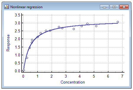
Scatter diagram & fitted line

This graph displays a scatter diagram and the fitted nonlinear regression line.

Residuals plot

Residuals are the differences between the predicted values and the observed values for the dependent variable.

The residuals plot allows for the visual evaluation of the goodness of fit of the model. Residuals may point to possible outliers (unusual values) in the data or problems with the fitted model. If the residuals display a certain pattern, the selected model may be inaccurate.

Literature

• Glantz SA, Slinker BK (2001) Primer of applied regression & analysis of variance. 2^nd ed. McGraw-Hill.
• Press WH, Teukolsky SA, Vetterling WT, Flannery BP (2007) Numerical Recipes. The Art of Scientific Computing. Third Edition. New York: Cambridge University Press.

See also

• Nonlinear regression worked example: example of a 4-parameter logistic model fit
• Regression
• Logistic regression
• Probit regression (Dose-Response analysis)

External links

• Levenberg–Marquardt algorithm on Wikipedia.