Nonlinear regression worked example: 4-parameter logistic model
Data
In this example we will fit a 4-parameter logistic model to the following data:

The equation for the 4-parameter logistic model is as follows:
 $$ \operatorname{F}(x) = d + \frac {a-d} { 1 + \left(\frac{x}{c} \right)^b } $$
which can be written as:
F(x) = d + ( a − d) / (1 + (x/c)^b)
where
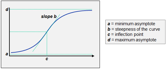
- a = Minimum asymptote. In a bioassay where you have a standard curve, this can be thought of as the response value at 0 standard concentration.
- b = Hill's slope. The Hill's slope refers to the steepness of the curve (can be positive or negative).
- c = Inflection point. The inflection point is defined as the point on the curve where the curvature changes direction or signs. C is the dose where y=(d-a)/2.
- d = Maximum asymptote. In a bioassay where you have a standard curve, this can be thought of as the response value for infinite standard concentration.
Scatter diagram
First we look at the scatter diagram with Response as dependent variable Y and Dose as independent variable X. In the scatter diagram, we want to plot a LOESS smoothed trendline. We complete the dialog box as follows:

This results in the following scatter diagram:

From this graph we will be able to estimate initial values for the parameters of the 4-parameter logistic model (see below).
Nonlinear regression
First we enter the regression equation d+(a-d)/(1+(x/c)^b) (we don't need to enter the 'y=' part) and select Response as dependent variable Y and Dose as independent variable X:

We leave the default values for Convergence tolerance and for Maximum number of iterations unchanged. We select the options to display a scatter diagram with fitted line and the residuals plot.
Initial parameters
We click and MedCalc extracts the parameter names from the equation: d, a, c and b:

We now need to enter initial values or best guesses for the different parameters. The scatter diagram above is useful for finding the following estimates:
- d is the upper asymptote and we guess it with the maximum value of the Response variable, which is about 25.
- a is the lower asymptote and we guess it with the minimum value of the Response variable, which is about 0.
- c is the inflection point (the dose where you have half of the max response) and we estimate its value to be 18 which is approximately the dose whose response is nearest to the mid response.
- b is the Hill's slope and we guess it with the slope of the line between first and last point. The slope is given by Δy/Δx or (24.2-0.1)/(52.2-0) which is approximately 0.5.
We can enter these numbers in the corresponding input fields:

Some helpful functions
MedCalc provides some useful functions which can provide a general solution for establishing initial parameter values:
- for d we take the maximum value of the Response variable, so we can use the formula VMAX(&Y). VMAX(variable) returns the maximum value of a variable. MedCalc will substitute the symbol &Y with the dependent Y-variable we have selected in the dialog box which is Response. So VMAX(&Y) will return the maximum value of the Response variable. See VMAX function.
- for a we take the minimum value of the Response variable, so we can use the formula VMIN(&Y). See VMIN function.
- c is approximately the dose whose response is nearest to the mid response. We can approximate this with the average of the Response variable, so we can use the formula VAVERAGE(&X). MedCalc will substitute the symbol &X with the independent X-variable we have selected in the dialog box which is Dose. So VAVERAGE(&X) will return the average value of the Dose variable. See VAVERAGE function.
- b is the slope and we can estimate it with the function VSLOPE(&X,&Y). See VSLOPE function.
We can enter these formulae in the corresponding input fields:

We are now ready to proceed and click OK.
Results
To find the model's parameters, MedCalc uses the Levenberg-Marquardt iterative procedure (Press et al., 2007), which yields the following results:

The result tables show that the procedures stopped after 72 iterations because the Convergence criterion was met, i.e. the software could not obtain a further reduction of the Residual standard deviation.
Next the initial parameters are listed: the formulae VMAX(&Y), VMIN(&Y), VAVERAGE(&X) and VSLOPE(&X,&Y) yielded the values 24.2, 0.1, 15.6778 and 0.5116 for d, a, c and b respectively, quite close to our own estimates based on the inspection of the scatter diagram, which were 25, 0, 18,and 0.5.
The program reports the sample size and the Residual standard deviation, followed with the regression equation and the calculated values of the regression parameters.
The inflection point c, for example, is estimated to be 19.3494 with Standard Error 0.5107 and 95% Confidence Interval 18.0365 to 20.6623.
The F-test that follows the Analysis of variance table shows a P-value of less than 0.0001. The F-test is an approximate test for the overall fit of the regression equation (Glantz & Slinker, 2001). A low P-value is an indication of a good fit.
Scatter diagram & fitted line
This graph displays a scatter diagram and the fitted nonlinear regression line, which shows that the fitted line corresponds well with the observed data:

Residuals plot
Our residuals plot does not show any outliers in the data and do not show a certain pattern. The residual plot therefore does not indicate a problem with our model.

Literature
- Glantz SA, Slinker BK (2001) Primer of applied regression & analysis of variance. 2nd ed. McGraw-Hill.
- Press WH, Teukolsky SA, Vetterling WT, Flannery BP (2007) Numerical Recipes. The Art of Scientific Computing. Third Edition. New York: Cambridge University Press.
