Logistic regression
| Command: | Statistics |
Description
Logistic regression is a statistical method for analyzing a dataset in which there are one or more independent variables that determine an outcome. The outcome is measured with a dichotomous variable (in which there are only two possible outcomes).
In logistic regression, the dependent variable is binary or dichotomous, i.e. it only contains data coded as 1 (TRUE, success, pregnant, etc.) or 0 (FALSE, failure, non-pregnant, etc.).
The goal of logistic regression is to find the best fitting (yet biologically reasonable) model to describe the relationship between the dichotomous characteristic of interest (dependent variable = response or outcome variable) and a set of independent (predictor or explanatory) variables. Logistic regression generates the coefficients (and its standard errors and significance levels) of a formula to predict a logit transformation of the probability of presence of the characteristic of interest:
where p is the probability of presence of the characteristic of interest. The logit transformation is defined as the logged odds:
and
Rather than choosing parameters that minimize the sum of squared errors (like in ordinary regression), estimation in logistic regression chooses parameters that maximize the likelihood of observing the sample values.
How to enter data
In the following example there are two predictor variables: AGE and SMOKING. The dependent variable, or response variable is OUTCOME. The dependent variable OUTCOME is coded 0 (negative) and 1 (positive).

Required input

Dependent variable
The variable whose values you want to predict. The dependent variable must be binary or dichotomous, and should only contain data coded as 0 or 1. If your data are coded differently, you can use the Define status tool to recode your data.
Independent variables
Select the different variables that you expect to influence the dependent variable.
Filter
(Optionally) enter a data filter in order to include only a selected subgroup of cases in the analysis.
Options
- Method: select the way independent variables are entered into the model.
- Enter: enter all variables in the model in one single step, without checking
- Forward: enter significant variables sequentially
- Backward: first enter all variables into the model and next remove the non-significant variables sequentially
- Stepwise: enter significant variables sequentially; after entering a variable in the model, check and possibly remove variables that became non-significant.
- Enter variable if P< A variable is entered into the model if its associated significance level is less than this P-value.
- Remove variable if P> A variable is removed from the model if its associated significance level is greater than this P-value.
- Classification table cutoff value: a value between 0 and 1 which will be used as a cutoff value for a classification table. The classification table is a method to evaluate the logistic regression model. In this table the observed values for the dependent outcome and the predicted values (at the selected cut-off value) are cross-classified.
- Categorical: click this button to identify categorical variables.
Graph
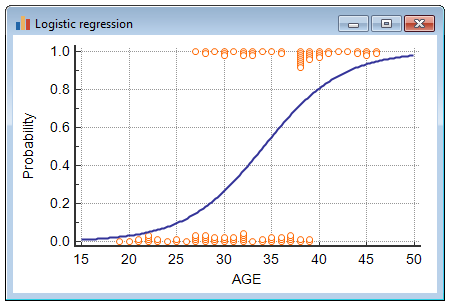
The option to plot a graph that shows the logistic regression curve is only available when there is just one single independent variable.
Results
After you click OK the following results are displayed:

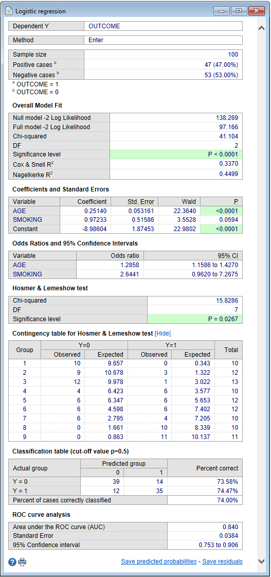
Sample size and cases with negative and positive outcome
First the program gives sample size and the number and proportion of cases with a negative (Y=0) and positive (Y=1) outcome.
Overall model fit
The null model −2 Log Likelihood is given by −2 * ln(L0) where L0 is the likelihood of obtaining the observations if the independent variables had no effect on the outcome.
The full model −2 Log Likelihood is given by −2 * ln(L) where L is the likelihood of obtaining the observations with all independent variables incorporated in the model.
The difference of these two yields a Chi-Squared statistic which is a measure of how well the independent variables affect the outcome or dependent variable.
If the P-value for the overall model fit statistic is less than the conventional 0.05 then there is evidence that at least one of the independent variables contributes to the prediction of the outcome.
Cox & Snell R2 and Nagelkerke R2 are other goodness of fit measures known as pseudo R-squared. Note that Cox & Snell's pseudo R-squared has a maximum value that is not 1. Nagelkerke R2 adjusts Cox & Snell's so that the range of possible values extends to 1.
Regression coefficients
The logistic regression coefficients are the coefficients b0, b1, b2, ... bk of the regression equation:
An independent variable with a regression coefficient not significantly different from 0 (P>0.05) can be removed from the regression model (press function key F7 to repeat the logistic regression procedure). If P<0.05 then the variable contributes significantly to the prediction of the outcome variable.
The logistic regression coefficients show the change (increase when bi>0, decrease when bi<0) in the predicted logged odds of having the characteristic of interest for a one-unit change in the independent variables.
When the independent variables Xa and Xb are dichotomous variables (e.g. Smoking, Sex) then the influence of these variables on the dependent variable can simply be compared by comparing their regression coefficients ba and bb.
The Wald statistic is the regression coefficient divided by its standard error squared: (b/SE)2.
Odds ratios with 95% CI
By taking the exponential of both sides of the regression equation as given above, the equation can be rewritten as:
It is clear that when a variable Xi increases by 1 unit, with all other factors remaining unchanged, then the odds will increase by a factor ebi.
This factor ebi is the "adjusted" odds ratio (O.R.) for the independent variable Xi and it gives the relative amount by which the odds of the outcome increase (O.R. greater than 1) or decrease (O.R. less than 1) when the value of the independent variable is increased by 1 units.
E.g. The variable SMOKING is coded as 0 (= no smoking) and 1 (= smoking), and the odds ratio for this variable is 2.64. This means that in the model the odds for a positive outcome in cases that do smoke are 2.64 times higher than in cases that do not smoke.
Interpretation of the fitted logistic regression equation
The logistic regression equation is:
So for 40 years old cases who do smoke logit(p) equals 2.026. Logit(p) can be back-transformed to p by the following formula:
Alternatively, you can use the Logit table or the ALOGIT function calculator. For logit(p)=2.026 the probability p of having a positive outcome equals 0.88.
Hosmer-Lemeshow test
The Hosmer-Lemeshow test is a statistical test for goodness of fit for the logistic regression model. The data are divided into approximately ten groups defined by increasing order of estimated risk. The observed and expected number of cases in each group is calculated and a Chi-squared statistic is calculated as follows:
with Og, Eg and ng the observed events, expected events and number of observations for the gth risk decile group, and G the number of groups. The test statistic follows a Chi-squared distribution with G−2 degrees of freedom.
A large value of Chi-squared (with small p-value < 0.05) indicates poor fit and small Chi-squared values (with larger p-value closer to 1) indicate a good logistic regression model fit.
The Contingency Table for Hosmer and Lemeshow Test table shows the details of the test with observed and expected number of cases in each group.
Classification table
The classification table is another method to evaluate the predictive accuracy of the logistic regression model. In this table the observed values for the dependent outcome and the predicted values (at a user defined cut-off value, for example p=0.50) are cross-classified. In our example, the model correctly predicts 74% of the cases.
ROC curve analysis
Another method to evaluate the logistic regression model makes use of ROC curve analysis. In this analysis, the power of the model's predicted values to discriminate between positive and negative cases is quantified by the Area under the ROC curve (AUC). The AUC, sometimes referred to as the C-statistic (or concordance index), is a value that varies from 0.5 (discriminating power not better than chance) to 1.0 (perfect discriminating power).
To perform a full ROC curve analysis on the predicted probabilities you can save the predicted probabilities and next use this new variable in ROC curve analysis. The Dependent variable used in Logistic Regression then acts as the Classification variable in the ROC curve analysis dialog box.
Propensity scores
Propensity scores are predicted probabilities of a logistic regression model. To save the propensity scores in your datasheet, click the link "Save predicted probabilities" in the results window.
Sample size considerations
Sample size calculation for logistic regression is a complex problem, but based on the work of Peduzzi et al. (1996) the following guideline for a minimum number of cases to include in your study can be suggested.
Let p be the smallest of the proportions of negative or positive cases in the population and k the number of covariates (the number of independent variables), then the minimum number of cases to include is:
N = 10 k / p
For example: you have 3 covariates to include in the model and the proportion of positive cases in the population is 0.20 (20%). The minimum number of cases required is
N = 10 x 3 / 0.20 = 150
If the resulting number is less than 100 you should increase it to 100 as suggested by Long (1997).
Graph
MedCalc can plot the logistic regression curve when there is only one single independent variable:

The following graph is created:

References
- Hosmer DW Jr, Lemeshow S, Sturdivant RX (2013) Applied Logistic Regression. Third Edition. New Jersey: John Wiley & Sons.
- Long JS (1997) Regression Models for categorical and limited dependent variables. Thousand Oaks, CA: Sage Publications.
- Pampel FC (2020) Logistic regression: A primer. Quantitative Applications in the Social Sciences, 132. Thousand Oaks, CA: Sage Publications.
- Peduzzi P, Concato J, Kemper E, Holford TR, Feinstein AR (1996) A simulation study of the number of events per variable in logistic regression analysis. Journal of Clinical Epidemiology 49:1373-1379.

