Probit regression (Dose-Response analysis)

Command:

Statistics Regression Probit regression (Dose-Response analysis)

Description

The probit regression procedure fits a probit sigmoid dose-response curve and calculates values (with 95% CI) of the dose variable that correspond to a series of probabilities. For example the ED50 (median effective dose) or (LD50 median lethal dose) are the values corresponding to a probability of 0.50, the Limit-of-Detection (CLSI, 2012) is the value corresponding to a probability of 0.95.

The probit regression equation has the form:

Where X is the (possibly log-transformed) dose variable and probit(p) is the value of the inverse standard normal cumulative distribution function Φ⁻¹ corresponding with a probability p:

Probit(p) can be transformed to a probability p using the standard normal cumulative distribution function Φ:

MedCalc fits the regression coefficients a and b using the method of maximum likelihood.

How to enter data

You can enter the data in binary format or in grouped format.

Binary

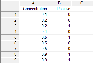
In the binary format, you have 2 variables, one variable for the dose (concentration) and one for the binary response.

For each single measurement, there is a row with the dose and the response, which is coded 0 (no response) and 1 (response).

For example:

Grouped

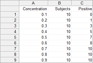
In the grouped format, you have 3 variables, one variable for the dose, one for the total number of measurements, and one for the number of measurements with a response.

For example:

Required input

Data type

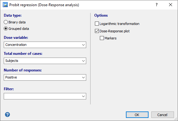
Select the option corresponding to the way you have entered the data: binary or grouped (see above).

Dose variable

Select the dose variable.

Variables in case of binary data

• Response variable: the response variable must be binary or dichotomous, and should only contain data coded as 0 (no response) or 1 (response). If your data are coded differently, you can use the Define status tool to recode your data.

Variables in case of grouped data

• Total number of cases: select the variable that contains the number of measurements for each dose.
• Number of responses: select the variable that contains the number of responses for each dose.

Filter

(Optionally) enter a data filter in order to include only a selected subgroup of cases in the analysis.

Options

• Log transformation: select this option if the dose variable requires a logarithmic transformation. When the dose variable contains 0 values, MedCalc will automatically add a small number to the data in order to make the logarithmic transformation possible. This small number will be subtracted when the results are back-transformed for presentation.
• Dose-response plot: select this option to obtain a dose-response plot.
  Markers: click this option to have the data represented in the graph as markers. Note that when you have selected logarithmic transformation and the dose variable contains 0 values, these values cannot be represented in the graph as markers.

Results

Sample size and cases with negative and positive outcome

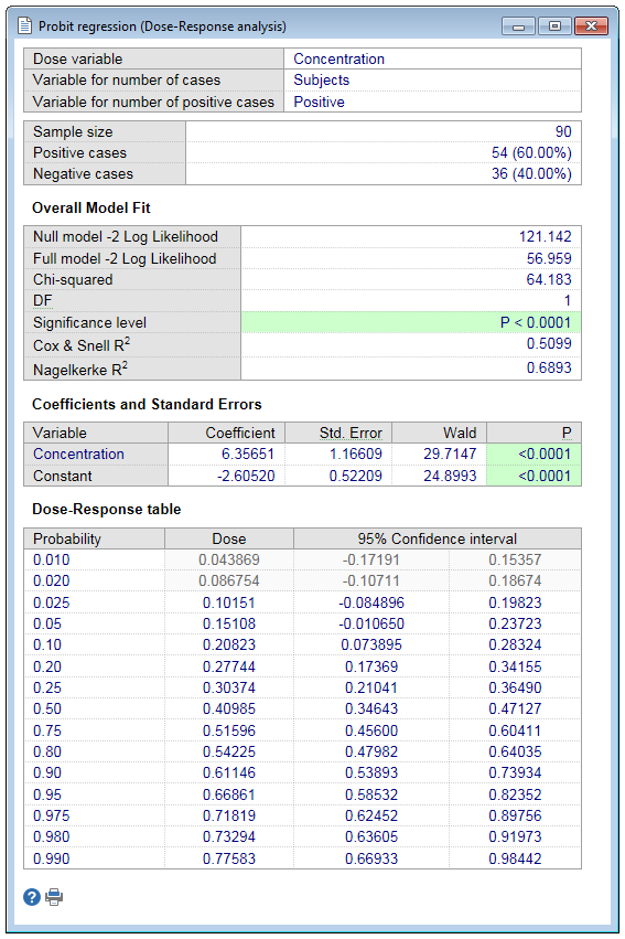
First the program gives sample size and the number and proportion of cases with and without response.

Overall model fit

The null model −2 Log Likelihood is given by −2 * ln(L₀) where L₀ is the likelihood of obtaining the observations in the "null" model, a model without the dose variable.

The full model −2 Log Likelihood is given by −2 * ln(L) where L is the likelihood of obtaining the observations with the dose variable incorporated in the model.

The difference of these two yields a Chi-Squared statistic which is a measure of how well the dose variable affects the response variable.

Cox & Snell R² and Nagelkerke R² are other goodness of fit measures known as pseudo R-squared. Note that Cox & Snell's pseudo R-squared has a maximum value that is not 1. Nagelkerke R² adjusts Cox & Snell's so that the range of possible values extends to 1.

Regression coefficients

The regression coefficients are the coefficients a (constant) and b (slope) of the regression equation:

The Wald statistic is the regression coefficient divided by its standard error squared: (b/SE)².

Log transformation

When you have selected logarithmic transformation of the dose variable, then a and b are in fact the coefficients of the regression equation:

Use of the fitted equation

The predicted probability of a positive response can be calculated using the regression equation.

When the regression equation is for example:

then for a Dose of 0.500 probit(p) equals 0.57. Probit(p) can be transformed to p by the MedCalc spreadsheet function NORMSDIST(z) or the equivalent Excel function.

Alternatively, you can use the following table.

Probit(p)	p
2.326	0.99
1.645	0.95
1.282	0.90
0.842	0.80
0.000	0.50
-0.842	0.20
-1.282	0.10
-1.645	0.05
-2.326	0.01

In the example, with probit(p) equal to 0.57, p = 0.72.

A probability p can be transformed to Probit(p) using the table above or using the MedCalc spreadsheet function NORMSINV(p) or the equivalent Excel function. For a probability p=0.5 you find in the table that probit(p)=0. When the regression equation is

probit = −2.61 + 6.36 × Dose

then

Dose = (probit+2.61)/6.36

and therefore dose = 2.61/6.36 = 0.41.

Dose-Response table

This table lists a series of Probabilities with corresponding Dose, with a 95% confidence interval for the dose (Finney, 1947).

Values in light gray text color are dose values that fall outside the observed range of the dose variable.

Log transformation

When you have selected logarithmic transformation of the dose variable, MedCalc back-transforms the results and displays the dose variable on its original scale in the Dose-Response table.

Graph

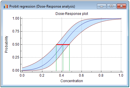
This graph shows the probabilities, ranging from 0 to 1, and the corresponding dose. Two additional curves represent the 95% confidence interval for the dose.

The dose and 95% confidence interval, corresponding with a particular probability, are taken from a horizontal line at that probability level.

Literature

• CLSI (2012) Evaluation of detection capability for clinical laboratory measurement procedures; Approved guideline - 2^nd edition. CLSI document EP17-A2. Wayne, PA: Clinical and Laboratory Standards Institute.
• Finney DJ (1947) Probit Analysis. A statistical treatment of the sigmoid response curve. Cambridge: Cambridge University Press.

See also

• Logistic regression
• Nonlinear regression

External links

• Probit model on Wikipedia.
• Median lethal dose on Wikipedia.