Regression
| Command: | Statistics |
Description
Regression analysis is a statistical method used to describe the relationship between two variables and to predict one variable from another (if you know one variable, then how well can you predict a second variable?).
Whereas for correlation the two variables need to have a Normal distribution, this is not a requirement for regression analysis. The variable X does not need to be a random sample with a Normal distribution (the values for X can be chosen by the experimenter). However, the variability of Y should be the same at each level of X.
Required input

Variables
- Variable Y and Variable X: select the dependent and independent variables Y and X.
- Weights: optionally select a variable containing relative weights that should be given to each observation (for weighted least-squares regression). Select the dummy variable "*** AutoWeight 1/SD^2 ***" for an automatic weighted regression procedure to correct for heteroscedasticity (Neter et al., 1996). This dummy variable appears as the first item in the drop-down list for Weights.
- Filter: you may also enter a data filter in order to include only a selected subgroup of cases in the statistical analysis.
Regression equation
By default the option Include constant in equation is selected. This is the recommended option that will result in ordinary least-squares regression. When you need regression through the origin (no constant a in the equation), you can uncheck this option (an example of when this is appropriate is given in Eisenhauer, 2003).
MedCalc offers a choice of 5 different regression equations:
| y | = | a + b x | straight line |
| y | = | a + b log(x) | logarithmic curve |
| log(y) | = | a + b x | exponential curve |
| log(y) | = | a + b log(x) | geometric curve |
| y | = | a + b x + c x2 | quadratic regression (parabola) |
where x represents the independent variable and y the dependent variable. The coefficients a, b and c are calculated by the program using the method of least squares.
Options
- Subgroups: allows to select a categorical variable containing codes to identify distinct subgroups. Regression analysis will be performed for all cases and for each subgroup.
- Residuals: you can select a Test for Normal distribution of the residuals.
Results
The following statistics will be displayed in the results window:
Dependent Y | WEIGHT |
|---|---|
Independent X | LENGTH |
Least squares regression
Sample size | 100 |
|---|---|
Coefficient of determination R2 | 0.1988 |
Residual standard deviation | 8.6253 |
Regression Equation
y = -54.5957 + 0.7476 x | |||||
Parameter | Coefficient | Std. Error | 95% CI | t | P |
|---|---|---|---|---|---|
Intercept | -54.5957 | 26.7084 | -107.5975 to -1.5938 | -2.0441 | 0.0436 |
Slope | 0.7476 | 0.1516 | 0.4468 to 1.0485 | 4.9312 | <0.0001 |
Analysis of Variance
Source | DF | Sum of Squares | Mean Square |
|---|---|---|---|
Regression | 1 | 1809.0613 | 1809.0613 |
Residual | 98 | 7290.7787 | 74.3957 |
F-ratio | 24.3167 |
|---|---|
Significance level | P<0.0001 |
| Save predicted values - Save residuals Scatter diagram with regression line |
Sample size: the number of data pairs n
Coefficient of determination R2: this is the proportion of the variation in the dependent variable explained by the regression model, and is a measure of the goodness of fit of the model. It can range from 0 to 1, and is calculated as follows:
 $$ R^2 = \frac {explained\ variation} {total\ variation} = \frac {\sum_{}^{}{(y_{est}-\bar{y})^2}} {\sum_{}^{}{(y-\bar{y})^2}} $$
where y are the observed values for the dependent variable, $\bar{y}$ is the average of the observed values and yest are predicted values for the dependent variable (the predicted values are calculated using the regression equation).
Note: MedCalc does not report the coefficient of determination in case of regression through the origin, because it does not offer a good interpretation of the regression through the origin model (see Eisenhauer, 2003).
Residual standard deviation: the standard deviation of the residuals (residuals = differences between observed and predicted values). It is calculated as follows:
 $$s_{res} = \sqrt{\frac{\sum_{}^{}{(y-y_{est})^2}}{n-2}} $$
The residual standard deviation is sometimes called the Standard error of estimate (Spiegel, 1961).
The equation of the regression curve: the selected equation with the calculated values for a and b (and for a parabola a third coefficient c). E.g. Y = a + b X
Next, the standard errors are given for the intercept (a) and the slope (b), followed by the t-value and the P-value for the hypothesis that these coefficients are equal to 0. If the P-values are low (e.g. less than 0.05), then you can conclude that the coefficients are different from 0.
Note that when you use the regression equation for prediction, you may only apply it to values in the range of the actual observations. E.g. when you have calculated the regression equation for height and weight for school children, this equation cannot be applied to adults.
Analysis of variance: the analysis of variance table divides the total variation in the dependent variable into two components, one which can be attributed to the regression model (labeled Regression) and one which cannot (labeled Residual). If the significance level for the F-test is small (less than 0.05), then the hypothesis that there is no (linear) relationship can be rejected.
Comparison of regression lines
When you have selected a subgroup in the regression dialog box MedCalc will automatically compare the slopes and intercepts of the regression equation obtained in the different subgroups.
This comparison is performed when
- there are 2 subgroups
- there is no weight variable
- a constant is included in the equation
The results window then includes the following table:
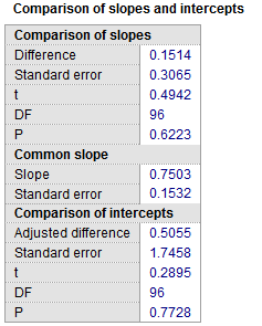
The calculations are performed according to Armitage et al., 2002.
First the difference between the slopes is reported with its standard error, t-statistic, degrees of freedom and associated P-value. If P is not less than 0.05 the slopes do not differ significantly and the regression lines are parallel. If P is less than 0.05 then the regression lines are not parallel and the comparison of intercepts below is not valid.
Next a common slope is calculated, which is used to calculate the adjusted difference between the intercepts.
This adjusted difference between the intercepts is reported with its standard error, t-statistic, degrees of freedom and associated P-value. If P is less than 0.05 there is a significant difference between the 2 intercepts. If P is not less than 0.05 then the two regression lines are indistinguishable.
Comparing regression lines using ANCOVA
When there are more than 2 subgroups, ANCOVA can be used to compare slopes and intercepts.
In the ANCOVA model you first select the dependent variable and next the independent variable is selected as a covariate. For Factors you select the grouping variable.
In the results for ANCOVA, below "Homogeneity of regression slopes" you will find a P-value which is the significance level for the comparison of the regression slopes. If this P-value is not less than 0.05 then the regression lines are parallel.
Next, below "Pairwise comparisons", you find the P-values for the differences between the intercepts.
Analysis of residuals
Linear regression analysis assumes that the residuals (the differences between the observations and the estimated values) follow a Normal distribution. This assumption can be evaluated with a formal test, or by means of graphical methods.
The different formal Tests for Normal distribution may not have enough power to detect deviation from the Normal distribution when sample size is small. On the other hand, when sample size is large, the requirement of a Normal distribution is less stringent because of the central limit theorem.
Therefore, it is often preferred to visually evaluate the symmetry and peakedness of the distribution of the residuals using the Histogram, Box-and-whisker plot, or Normal plot.
To do so, you click the hyperlink "Save residuals" in the results window. This will save the residual values as a new variable in the spreadsheet. You can then use this new variable in the different distribution plots.
Presentation of results
If the analysis shows that the relationship between the two variables is too weak to be of practical help, then there is little point in quoting the equation of the fitted line or curve. If you give the equation, you also report the standard error of the slope, together with the corresponding P-value. Also the residual standard deviation should be reported (Altman, 1980). The number of decimal places of the regression coefficients should correspond to the precision of the raw data.
The accompanying scatter diagram should include the fitted regression line when this is appropriate. This figure can also include the 95% confidence interval, or the 95% prediction interval, which can be more informative, or both. The legend of the figure must clearly identify the interval that is represented.
Literature
- Altman DG (1980) Statistics and ethics in medical research. VI - Presentation of results. British Medical Journal 281:1542-1544.

- Armitage P, Berry G, Matthews JNS (2002) Statistical methods in medical research. 4th ed. Blackwell Science.
- Bland M (2000) An introduction to medical statistics, 3rd ed. Oxford: Oxford University Press.
- Eisenhauer JG (2003) Regression through the origin. Teaching Statistics 25:76-80.
- Neter J, Kutner MH, Nachtsheim CJ, Wasserman W (1996) Applied linear statistical models. 4th ed. Boston: McGraw-Hill.
