ROC curve analysis
| Command: | Statistics |
What is a ROC curve?
A ROC curve is a plot of the true positive rate (Sensitivity) in function of the false positive rate (100-Specificity) for different cut-off points of a parameter. Each point on the ROC curve represents a sensitivity/specificity pair corresponding to a particular decision threshold. The Area Under the ROC curve (AUC) is a measure of how well a parameter can distinguish between two diagnostic groups (diseased/normal).
MedCalc creates a complete sensitivity/specificity report.
The ROC curve is a fundamental tool for diagnostic test evaluation.
Theory summary
The diagnostic performance of a test, or the accuracy of a test to discriminate diseased cases from normal cases is evaluated using Receiver Operating Characteristic (ROC) curve analysis (Metz, 1978; Zweig & Campbell, 1993). ROC curves can also be used to compare the diagnostic performance of two or more laboratory or diagnostic tests (Griner et al., 1981).
When you consider the results of a particular test in two populations, one population with a disease, the other population without the disease, you will rarely observe a perfect separation between the two groups. Indeed, the distribution of the test results will overlap, as shown in the following figure.

For every possible cut-off point or criterion value you select to discriminate between the two populations, there will be some cases with the disease correctly classified as positive (TP = True Positive fraction), but some cases with the disease will be classified negative (FN = False Negative fraction). On the other hand, some cases without the disease will be correctly classified as negative (TN = True Negative fraction), but some cases without the disease will be classified as positive (FP = False Positive fraction).
Schematic outcomes of a test
The different fractions (TP, FP, TN, FN) are represented in the following table.
| Disease | |||||||
| Test | Present | n | Absent | n | Total | ||
| Positive | True Positive (TP) | a | False Positive (FP) | c | a + c | ||
| Negative | False Negative (FN) | b | True Negative (TN) | d | b + d | ||
| Total | a + b | c + d |
The following statistics can be defined:
| Sensitivity |
|
Specificity |
|
|||||
| Positive Likelihood Ratio |
|
Negative Likelihood Ratio |
|
|||||
| Positive Predictive Value |
|
Negative Predictive Value |
|
- Sensitivity: probability that a test result will be positive when the disease is present (true positive rate, expressed as a percentage).
$$ Sensitivity = \frac { a } { a + b} $$
- Specificity: probability that a test result will be negative when the disease is not present (true negative rate, expressed as a percentage).
$$ Specificity = \frac { d } { c + d} $$
- Positive likelihood ratio: ratio between the probability of a positive test result given the presence of the disease and the probability of a positive test result given the absence of the disease, i.e.
$$ +LR = \frac { True\ positive\ rate } { False\ positive\ rate } = \frac { Sensitivity} { 1 - Specificity} $$
- Negative likelihood ratio: ratio between the probability of a negative test result given the presence of the disease and the probability of a negative test result given the absence of the disease, i.e.
$$ -LR = \frac { False\ negative\ rate } { True\ negative\ rate } = \frac { 1 - Sensitivity} { Specificity} $$
- Positive predictive value: probability that the disease is present when the test is positive (expressed as a percentage).
$$ PPV = \frac { a } { a + c} $$
- Negative predictive value: probability that the disease is not present when the test is negative (expressed as a percentage).
$$ NPV = \frac { d } { b + d} $$
Sensitivity and specificity versus criterion value
When you select a higher criterion value, the false positive fraction will decrease with increased specificity but on the other hand the true positive fraction and sensitivity will decrease:

When you select a lower threshold value, then the true positive fraction and sensitivity will increase. On the other hand the false positive fraction will also increase, and therefore the true negative fraction and specificity will decrease.
The ROC curve
In a Receiver Operating Characteristic (ROC) curve the true positive rate (Sensitivity) is plotted in function of the false positive rate (100-Specificity) for different cut-off points. Each point on the ROC curve represents a sensitivity/specificity pair corresponding to a particular decision threshold. A test with perfect discrimination (no overlap in the two distributions) has a ROC curve that passes through the upper left corner (100% sensitivity, 100% specificity). Therefore the closer the ROC curve is to the upper left corner, the higher the overall accuracy of the test (Zweig & Campbell, 1993).

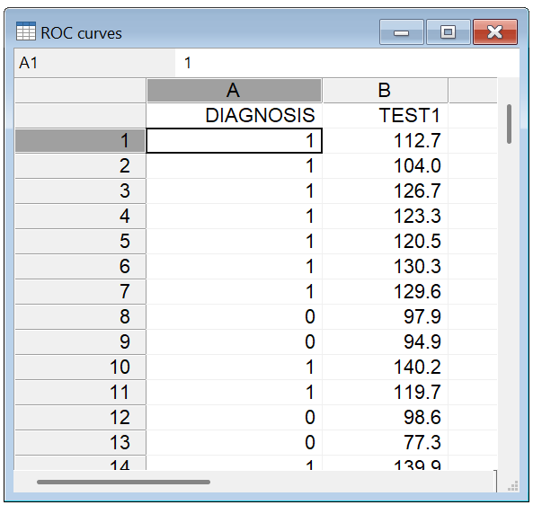
How to enter data for ROC curve analysis
In order to perform ROC curve analysis in MedCalc you should have a measurement of interest (= the parameter you want to study) and an independent diagnosis which classifies your study subjects into two distinct groups: a diseased and non-diseased group. The latter diagnosis should be independent from the measurement of interest.
In the spreadsheet, create a column DIAGNOSIS and a column for the variable of interest, e.g. TEST1. For every study subject enter a code for the diagnosis as follows: 1 for the diseased cases, and 0 for the non-diseased or normal cases. In the TEST1 column, enter the measurement of interest (this can be measurements, grades, etc. - if the data are categorical, code them with numerical values).
Required input
Complete the ROC curve analysis dialog box as follows:

Data
- Variable: select the variable of interest. This variable contains the results of the diagnostic test which for which you want to obtain the test characteristics.
- Classification variable: select or enter a dichotomous variable indicating diagnosis (0=negative, 1=positive).If your data are coded differently, you can use the Define status tool to recode your data.
- Filter: (optionally) a filter in order to include only a selected subgroup of cases (e.g. AGE>21, SEX="Male").
Methodology
- DeLong et al.: use the method of DeLong et al. (1988) for the calculation of the Standard Error of the Area Under the Curve (recommended).
- Hanley & McNeil: use the method of Hanley & McNeil (1982) for the calculation of the Standard Error of the Area Under the Curve.
- Binomial exact Confidence Interval for the AUC: calculate an exact Binomial Confidence Interval for the Area Under the Curve (recommended). If this option is not selected, the Confidence Interval is calculated as AUC ± 1.96 its Standard Error.
Disease prevalence
Whereas sensitivity and specificity, and therefore the ROC curve, and positive and negative likelihood ratio are independent of disease prevalence, positive and negative predictive values are highly dependent on disease prevalence or prior probability of disease. Therefore when disease prevalence is unknown, the program cannot calculate positive and negative predictive values.
Clinically, the disease prevalence is the same as the probability of disease being present before the test is performed (prior probability of disease).
- Unknown: select this option when the disease prevalence is unknown, or irrelevant for the current statistical analysis.
- The ratio of cases in the positive and negative groups reflects the prevalence of the disease: if the sample sizes in the positive and the negative group reflect the real prevalence of the disease in the population, this can be indicated by selecting this option.
- Other value (%): alternatively you can enter a value for the disease prevalence, expressed as a percentage.
Options
- List criterion values with test characteristics: option to create a list of criterion values corresponding with the coordinates of the ROC curve, with associated sensitivity, specificity, likelihood ratios and predictive values (if disease prevalence is known).
- Include all observed criterion values: When you select this option, the program will list sensitivity and specificity for all possible threshold values. If this option is not selected, then the program will only list the more important points of the ROC curve: for equal sensitivity/specificity it will give the threshold values (criterion values) with the highest specificity/sensitivity.
- 95% Confidence Interval for sensitivity/specificity, likelihood ratio and predictive values: select the Confidence Intervals you require.
- Calculate optimal criterion value taking into account costs: option to calculate the optimal criterion value taking into account the disease prevalence and cost of false and true positive and negative decisions (Zweig & Campbell, 1993). This option is only available if disease prevalence is known (see above).
- FPc: the cost of a false positive decision.
- FNc: the cost of a false negative decision.
- TPc: the cost of a true positive decision.
- TNc: the cost of a true negative decision.
$$ S = \left ( \frac {FP_c - TN_c} {FN_c - TP_c} \right ) \times \left ( \frac {1-P} {P} \right ) $$where P denotes the prevalence in the target population (Greiner et al., 2000). The point on the ROC curve where a line with this slope S touches the curve is the optimal operating point, taking into account prevalence and the costs of the different decisions.Costs can be financial costs or health costs, but all 4 cost factors need to be expressed on a common scale. Benefits can be expressed as negative costs. Suppose a false negative (FN) decision is judged to be twice as costly as a false positive (FP) decision, and no assumptions are made about the costs for true positive and true negative decisions. Then for FNc you enter 2, for FPc enter 1 and enter 0 for both TPc and TNc.
Because the slope S must be a positive number:
- FPc cannot be equal to TNc
- FNc cannot be equal to TPc
- When TNc is larger than FPc then TPc must be larger than FNc
- When TNc is smaller than FPc then TPc must be smaller than FNc
The parameter S is "cost-neutral" when (FPc-TNc)/(FNc-TPc) evaluates to 1, that is when FPc-TNc equals FNc-TPc. In this case S, and the "optimal criterion value" depends only on the disease prevalence.
- Advanced: click this button for some advanced options:
These options require bootstrapping and are computationally intensive and time consuming.
- Estimation of sensitivity and specificity at fixed specificity and sensitivity: compile a table with estimation of sensitivity and specificity, with a BCa bootstrapped 95% confidence interval (Efron, 1987; Efron & Tibshirani, 1993), for a fixed and prespecified specificity and sensitivity of 80%, 90%, 95% and 97.5% (Zhou et al., 2002).
- Bootstrap Youden index confidence interval: calculate a BCa bootstrapped 95% confidence interval for the Youden index and its associated criterion value.
- Bootstrap replications: enter the number of bootstrap replications. 1000 replications is a number commonly encountered in the literature. High numbers increase accuracy but also increase processing time.
- Random-number seed: this is the seed for the random number generator. Enter 0 for a random seed; this can result in different confidence intervals when the procedure is repeated. Any other value will give a repeatable "random" sequence, which will result in repeatable values for the confidence intervals.
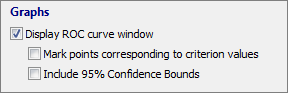
ROC graph
- Select Display ROC curve window to obtain the graph in a separate window.
Options:
- mark points corresponding to criterion values.
- display 95% Confidence Bounds for the ROC curve (Hilgers, 1991).
Results and interpretation of ROC curves
Sample size
First the program displays the number of observations in the two groups. Concerning sample size, it has been suggested that meaningful qualitative conclusions can be drawn from ROC experiments performed with a total of about 100 observations (Metz, 1978).
Variable | TEST1 |
|---|---|
Classification variable | DIAGNOSIS |
| Sample size | 100 |
|---|---|
Positive group a | 55 (55.00%) |
Negative group b | 45 (45.00%) |
a DIAGNOSIS = 1
b DIAGNOSIS = 0
Disease prevalence (%) | 10 |
|---|
Area under the ROC curve
MedCalc reports the Area under the ROC curve with standard error and 95% Confidence Interval.
Area under the ROC curve (AUC)
Area under the ROC curve (AUC) | 0.947 |
|---|---|
Standard Error a | 0.0241 |
95% Confidence interval b | 0.883 to 0.982 |
z statistic | 18.544 |
Significance level P (Area=0.5) | <0.0001 |
a DeLong et al., 1988
b Binomial exact
The Area under the ROC curve (AUC) can be interpreted as follows (Zhou, Obuchowski & McClish, 2002):
- the average value of sensitivity for all possible values of specificity;
- the average value of specificity for all possible values of sensitivity;
- the probability that a randomly selected individual from the positive group has a test result indicating greater suspicion than that for a randomly chosen individual from the negative group.
When the variable under study cannot distinguish between the two groups, i.e. where there is no difference between the two distributions, the area will be equal to 0.5 (the ROC curve will coincide with the diagonal). When there is a perfect separation of the values of the two groups, i.e. there no overlapping of the distributions, the area under the ROC curve equals 1 (the ROC curve will reach the upper left corner of the plot).
The 95% Confidence Interval is the interval in which the true (population) Area under the ROC curve lies with 95% confidence.
The Significance level or P-value is the probability that the observed sample Area under the ROC curve is found when in fact, the true (population) Area under the ROC curve is 0.5 (null hypothesis: Area = 0.5). If P is small (P<0.05) then it can be concluded that the Area under the ROC curve is significantly different from 0.5 and that therefore there is evidence that the laboratory test does have an ability to distinguish between the two groups (Hanley & McNeil, 1982; Zweig & Campbell, 1993).
Youden index
The Youden index is reported with its 95% confidence interval and associated criterion.
Youden index
Youden index J | 0.8202 |
|---|---|
95% Confidence interval a | 0.6979 to 0.9051 |
Associated criterion | >108.9 |
95% Confidence interval a | >107.9 to >114.8 |
Sensitivity | 90.91 |
Specificity | 91.11 |
a BCa bootstrap confidence interval (1000 iterations; random number seed: 978).
The Youden index J (Youden, 1950) is defined as:
where c ranges over all possible criterion values.
Graphically, J is the maximum vertical distance between the ROC curve and the diagonal line.
The criterion value corresponding with the Youden index J is the optimal criterion value only when disease prevalence is 50%, equal weight is given to sensitivity and specificity, and costs of various decisions are ignored.
When the corresponding Advanced option has been selected, MedCalc will calculate BCa bootstrapped 95% confidence intervals (Efron, 1987; Efron & Tibshirani, 1993) for both the Youden index and it's corresponding criterion value.
Criterion values
MedCalc does not simply reports threshold or criterion values, but it reports the criterion values with a comparison sign, > or ≤, depending on whether higher values indicate disease, of lower values indicate disease.
See the note on Criterion values.
Optimal criterion
This panel is only displayed when disease prevalence and cost parameters are known.
Optimal criterion
Optimal criterion a | >114.8 |
|---|---|
95% Confidence interval b | >112.9 to >114.8 |
Sensitivity | 76.36 |
Specificity | 97.78 |
a Taking into account disease prevalence (10%) and estimated costs:
cost False Positive: 1; cost False Negative: 2
cost True Positive: 0; cost True Negative: 0
b BCa bootstrap confidence interval (1000 iterations; random number seed: 978).
The optimal criterion value takes into account not only sensitivity and specificity, but also disease prevalence, and costs of various decisions. When these data are known, MedCalc will calculate the optimal criterion and associated sensitivity and specificity. And when the corresponding Advanced option has been selected, MedCalc will calculate BCa bootstrapped 95% confidence intervals (Efron, 1987; Efron & Tibshirani, 1993) for these parameters.
When a test is used either for the purpose of screening or to exclude a diagnostic possibility, a cut-off value with a higher sensitivity may be selected; and when a test is used to confirm a disease, a higher specificity may be required.
Summary table
This panel is only displayed when the corresponding Advanced option has been selected.
The summary table displays the estimated specificity for fixed and prespecified sensitivities of 80, 90, 95 and 97.5% as well as estimated sensitivity for fixed and prespecified specificities (Zhou et al., 2002), with the corresponding criterion values.
Summary Table
Estimated specificity at fixed sensitivity | |||
Sensitivity | Specificity | 95% CI a | Criterion |
|---|---|---|---|
80.00 | 95.56 | 84.44 to 100.00 | >112.9 |
90.00 | 91.11 | 68.89 to 100.00 | >109.45 |
95.00 | 73.33 | 32.15 to 94.77 | >103.8 |
97.50 | 66.67 | 24.44 to 86.67 | >102.575 |
99.00 | 37.78 | 15.56 to 66.67 | >94.955 |
Estimated sensitivity at fixed specificity | |||
Specificity | Sensitivity | 95% CI a | Criterion |
80.00 | 92.73 | 74.14 to 98.18 | >106.9 |
90.00 | 91.36 | 76.36 to 98.90 | >108.75 |
95.00 | 80.00 | 10.91 to 94.63 | >112.85 |
97.50 | 76.36 | 0.00 to 0.00 | >114.775 |
99.00 | 14.55 | 0.00 to 0.00 | >133.265 |
a BCa bootstrap confidence interval (1000 iterations; random number seed: 978).
Confidence intervals are BCa bootstrapped 95% confidence intervals (Efron, 1987; Efron & Tibshirani, 1993).
Criterion values and coordinates of the ROC curve
This section of the results window lists the different filters or cut-off values with their corresponding sensitivity and specificity of the test, and the positive (+LR) and negative likelihood ratio (-LR). When the disease prevalence is known, the program will also report the positive predictive value (+PV) and the negative predictive value (-PV).
Criterion values and coordinates of the ROC curve
Criterion | Sensitivity | 95% CI | Specificity | 95% CI | +LR | -LR | +PV | -PV | Cost |
|---|---|---|---|---|---|---|---|---|---|
≥77.3 | 100.00 | 93.5 - 100.0 | 0.00 | 0.0 - 7.9 | 1.00 |
| 10.0 |
| 0.900 |
>94.9 | 100.00 | 93.5 - 100.0 | 37.78 | 23.8 - 53.5 | 1.61 | 0.00 | 15.2 | 100.0 | 0.560 |
>95 | 98.18 | 90.3 - 100.0 | 37.78 | 23.8 - 53.5 | 1.58 | 0.048 | 14.9 | 99.5 | 0.564 |
>102.5 | 98.18 | 90.3 - 100.0 | 66.67 | 51.0 - 80.0 | 2.95 | 0.027 | 24.7 | 99.7 | 0.304 |
>102.7 | 96.36 | 87.5 - 99.6 | 66.67 | 51.0 - 80.0 | 2.89 | 0.055 | 24.3 | 99.4 | 0.307 |
>103.2 | 96.36 | 87.5 - 99.6 | 73.33 | 58.1 - 85.4 | 3.61 | 0.050 | 28.6 | 99.5 | 0.247 |
>104 | 94.55 | 84.9 - 98.9 | 73.33 | 58.1 - 85.4 | 3.55 | 0.074 | 28.3 | 99.2 | 0.251 |
>104.5 | 94.55 | 84.9 - 98.9 | 75.56 | 60.5 - 87.1 | 3.87 | 0.072 | 30.1 | 99.2 | 0.231 |
>104.9 | 92.73 | 82.4 - 98.0 | 75.56 | 60.5 - 87.1 | 3.79 | 0.096 | 29.7 | 98.9 | 0.235 |
>108.3 | 92.73 | 82.4 - 98.0 | 86.67 | 73.2 - 94.9 | 6.95 | 0.084 | 43.6 | 99.1 | 0.135 |
>108.9 | 90.91 | 80.0 - 97.0 | 91.11 | 78.8 - 97.5 | 10.23 | 0.100 | 53.2 | 98.9 | 0.0982 |
>110.7 | 81.82 | 69.1 - 90.9 | 91.11 | 78.8 - 97.5 | 9.20 | 0.20 | 50.6 | 97.8 | 0.116 |
>112.2 | 81.82 | 69.1 - 90.9 | 93.33 | 81.7 - 98.6 | 12.27 | 0.19 | 57.7 | 97.9 | 0.0964 |
>112.7 | 80.00 | 67.0 - 89.6 | 93.33 | 81.7 - 98.6 | 12.00 | 0.21 | 57.1 | 97.7 | 0.1000 |
>112.9 | 80.00 | 67.0 - 89.6 | 95.56 | 84.9 - 99.5 | 18.00 | 0.21 | 66.7 | 97.7 | 0.0800 |
>114.6 | 76.36 | 63.0 - 86.8 | 95.56 | 84.9 - 99.5 | 17.18 | 0.25 | 65.6 | 97.3 | 0.0873 |
>114.8 | 76.36 | 63.0 - 86.8 | 97.78 | 88.2 - 99.9 | 34.36 | 0.24 | 79.2 | 97.4 | 0.0673 |
>133.1 | 14.55 | 6.5 - 26.7 | 97.78 | 88.2 - 99.9 | 6.55 | 0.87 | 42.1 | 91.1 | 0.191 |
>133.4 | 14.55 | 6.5 - 26.7 | 100.00 | 92.1 - 100.0 |
| 0.85 | 100.0 | 91.3 | 0.171 |
>143.6 | 0.00 | 0.0 - 6.5 | 100.00 | 92.1 - 100.0 |
| 1.00 |
| 90.0 | 0.200 |
When you did not select the option Include all observed criterion values, the program only lists the more important points of the ROC curve: for equal sensitivity (resp. specificity) it gives the threshold value (criterion value) with the highest specificity (resp. sensitivity). When you do select the option Include all observed criterion values, the program will list sensitivity and specificity for all possible threshold values.
- Sensitivity (with optional 95% Confidence Interval): Probability that a test result will be positive when the disease is present (true positive rate).
- Specificity (with optional 95% Confidence Interval): Probability that a test result will be negative when the disease is not present (true negative rate).
- Positive likelihood ratio (with optional 95% Confidence Interval): Ratio between the probability of a positive test result given the presence of the disease and the probability of a positive test result given the absence of the disease.
- Negative likelihood ratio (with optional 95% Confidence Interval): Ratio between the probability of a negative test result given the presence of the disease and the probability of a negative test result given the absence of the disease.
- Positive predictive value (with optional 95% Confidence Interval): Probability that the disease is present when the test is positive.
- Negative predictive value (with optional 95% Confidence Interval): Probability that the disease is not present when the test is negative.
- Cost*: The average cost resulting from the use of the diagnostic test at that decision level. Note that the cost reported here excludes the "overhead cost", i.e. the cost of doing the test, which is constant at all decision levels. *This column is only displayed when disease prevalence and cost parameters are known.
Sensitivity, specificity, positive and negative predictive value as well as disease prevalence are expressed as percentages.
Confidence intervals for sensitivity and specificity are "exact" Clopper-Pearson confidence intervals.
Confidence intervals for the likelihood ratios are calculated using the "Log method" as given on page 109 of Altman et al. 2000.
Confidence intervals for the predictive values are the standard logit confidence intervals given by Mercaldo et al. 2007.
ROC curve
The ROC curve will be displayed in a second window when you have selected the corresponding option in the dialog box.
In a ROC curve the true positive rate (Sensitivity) is plotted in function of the false positive rate (100-Specificity) for different cut-off points. Each point on the ROC curve represents a sensitivity/specificity pair corresponding to a particular decision threshold. A test with perfect discrimination (no overlap in the two distributions) has a ROC curve that passes through the upper left corner (100% sensitivity, 100% specificity). Therefore the closer the ROC curve is to the upper left corner, the higher the overall accuracy of the test (Zweig & Campbell, 1993).

When you click on a specific point of the ROC curve, the corresponding cut-off point with sensitivity and specificity will be displayed.

This is the ROC curve with the option Include 95% Confidence Bounds:

Presentation of results
The prevalence of a disease may be different in different clinical settings. For instance the pre-test probability for a positive test will be higher when a patient consults a specialist than when he consults a general practitioner. Since positive and negative predictive values are sensitive to the prevalence of the disease, it would be misleading to compare these values from different studies where the prevalence of the disease differs, or apply them in different settings.
The data from the results window can be summarized in a table. The sample size in the two groups should be clearly stated. The table can contain a column for the different criterion values, the corresponding sensitivity (with 95% CI), specificity (with 95% CI), and possibly the positive and negative predictive value. The table should not only contain the test's characteristics for one single cut-off value, but preferably there should be a row for the values corresponding with a sensitivity of 90%, 95% and 97.5%, specificity of 90%, 95% and 97.5%, and the value corresponding with the Youden index or highest accuracy.
With these data, any reader can calculate the negative and positive predictive value applicable in his own clinical setting when the knows the prior probability of disease (pre-test probability or prevalence of disease) in this setting, by the following formulas based on Bayes' theorem:
and
The negative and positive likelihood ratio must be handled with care because they are easily and commonly misinterpreted.
Literature
- DeLong ER, DeLong DM, Clarke-Pearson DL (1988) Comparing the areas under two or more correlated receiver operating characteristic curves: a non-parametric approach. Biometrics 44:837-845.

- Efron B (1987) Better Bootstrap Confidence Intervals. Journal of the American Statistical Association 82:171-185.
- Efron B, Tibshirani RJ (1993) An introduction to the Bootstrap. Chapman & Hall/CRC.
- Greiner M, Pfeiffer D, Smith RD (2000) Principles and practical application of the receiver-operating characteristic analysis for diagnostic tests. Preventive Veterinary Medicine 45:23-41.
- Griner PF, Mayewski RJ, Mushlin AI, Greenland P (1981) Selection and interpretation of diagnostic tests and procedures. Annals of Internal Medicine 94:555-600.
- Hanley JA, Hajian-Tilaki KO (1997) Sampling variability of non-parametric estimates of the areas under receiver operating characteristic curves: an update. Academic Radiology 4:49-58.
- Hanley JA, McNeil BJ (1982) The meaning and use of the area under a receiver operating characteristic (ROC) curve. Radiology 143:29-36.
- Hilgers RA (1991) Distribution-free confidence bounds for ROC curves. Methods of Information in Medicine 30:96-101.
- Mercaldo ND, Lau KF, Zhou XH (2007) Confidence intervals for predictive values with an emphasis to case-control studies. Statistics in Medicine 26:2170-2183.
- Metz CE (1978) Basic principles of ROC analysis. Seminars in Nuclear Medicine 8:283-298.
- Youden WJ (1950) An index for rating diagnostic tests. Cancer 3:32-35.
- Zhou XH, Obuchowski NA, McClish DK (2002) Statistical methods in diagnostic medicine. Wiley-Interscience.
- Zweig MH, Campbell G (1993) Receiver-operating characteristic (ROC) plots: a fundamental evaluation tool in clinical medicine. Clinical Chemistry 39:561-577.
