Reference interval

Command:

Statistics Reference intervals Reference interval

Description

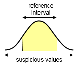
A Reference interval (Reference range, Normal range) for a parameter is the interval in which the central 95% values of apparently healthy subjects lie. For a double sided reference interval, where both low and high values are suspicious, there are 2 limits of normality: a lower limit (with 2.5% of healthy subjects below), and upper limit of normality (with 2.5% of subjects above that value).

When only low values are suspicious, then there is only a lower limit of normality (with 5% of healthy subjects beloww that value) and no upper limit of normality. This is a left sided reference interval.

On the other hand, when only high values are suspicious, then there is only a higher limit of normality (with 5% of healthy subjects above that value) and no upper limit of normality. This defines a right sided reference interval.

A 90% confidence interval (as recommended by the CLSI Guidelines C28-A3) is calculated for both limits of normality. As always, the confidence interval will be more narrow with higher number of subjects in the study, meaning more certainty about the reference limits.

The reference interval can be calculated using the following 3 methods: (a) using the Normal distribution (b) using a non-parametrical percentile method, and (c) optionally the robust method as described in the CLSI Guidelines C28-A3.

Normal distribution method

In the Normal distribution method, the mean, variance, and standard deviation of the sample data are calculated.

For a 2-sided reference interval, the limits of normality are :

The 90% confidence interval for each limit is given by (Bland, 2000):

The normal distribution method requires that the data present a normal distribution, possibly after logarithmic or Box-Cox transformation.

This method does not require a minimum number of subjects, but a minimum sample size of 40 is recommended (Le Boedic, 2019).

Percentile method

In the percentile method, the lower and upper limits of normality are given by the 2.5th and 97.5th percentiles for a double sided reference interval. The 5th percentile for a left sided reference interval, and 95th percentile for a right sided reference interval.

Following the CLSI guidelines, 90% confidence intervals are defined using the method of Reed et al. (1971).

For the calculation of a 90% confidence interval in the percentile method, a minimal sample size of 120 is required (CLSI, 2008).

Robust method

The calculation of a reference interval using the robust method (Horn & Pesce, 2005) involves an iterative process, in which the initial central value is estimated by the median and the initial spread by the median absolute deviation about the median (MAD). In the iterative process, actual observations are downweighted according to their distance from the central tendency of the sample. In each iteration, a quantity T_bi, representing the updated estimate of central tendency, is calculated, until the change in consecutive iterative values is negligible. Weighted estimators of variability and spread are calculated to establish the reference limits. See Horn & Pesce (2005) or CLSI (2008) for computational details.

90% confidence intervals for the reference limits are estimated using bootstrapping (percentile interval method, Efron & Tibshirani, 1993)

The robust method can be used as an alternative to the percentile method when sample size is less than 120.

Required input

In the dialog box you identify the variable with the measurements. You can click the button to obtain a list of variables. In this list you can select a variable by clicking the variable's name. You can also enter or select a filter in order to include only a selected subgroup of measurements in the statistical procedure, as described in the Introduction part of this manual.

Options

• Reference interval: you can select a 90%, 95%, 99%, 99.9%, or 99.99% reference interval. A 95% interval is the most usual and preferred setting.
• Double sided, left or right sided

  	Select Double sided when there is both a lower and upper limit of normality (both low and high values are suspicious)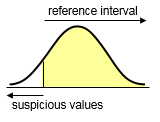
  	Select Left sided when there is only a lower limit of normality and no upper limit of normality (only low values are suspicious)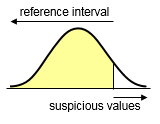
  	Select Right sided when there is only an upper limit of normality and no lower limit of normality (only high values are suspicious)

• Test for outliers: select the method based on Reed et al. (1971) or Tukey (1977) to automatically check the measurements for outliers (alternatively select none for no outlier testing). The method by Reed et al. will test only the minimum and maximum observations; the Tukey test can identify more values as outliers. The tests will create a list of possible outlying observations, but these will not automatically be excluded from the analysis. The possible outliers should be inspected by the investigator who can decide to exclude the values (see Exclude & Include).
  For other methods for outlier detection see Outlier detection.
• Follow CLSI guidelines for percentiles and their CIs: select this option to follow the NCCLS and Clinical and Laboratory Standards Institute (CLSI) guidelines C28-A2 and C28-A3 for estimating percentiles and their 90% confidence intervals. In these guidelines, percentiles are calculated as the observations corresponding to rank r=p*(n+1). Also for the 90% confidence intervals of the reference limits the CLSI guidelines are followed and conservative confidence intervals are calculated using integer ranks (and therefore the confidence intervals are at least 90% wide).
  If you do not select this option, MedCalc calculates percentiles as the observations corresponding to rank r=p*n+0.5 (Lentner, 1982; Schoonjans et al., 2011), and calculates a less conservative and more precise confidence interval using an iterative method.
• Robust method: select this option to calculate the reference limits with the "robust method" (CLSI Guidelines C28-A3). Recommended for smaller sample sizes (less than 120).

  With the Robust method, the confidence intervals for the reference limits are estimated using bootstrapping (percentile interval method, Efron & Tibshirani, 1993). Click Advanced... for bootstrapping options such as number of replications and random-number seed.

• Logarithmic transformation: if the data require a logarithmic transformation (e.g. when the data are positively skewed), select the Logarithmic transformation option.
• Box-Cox transformation: this will allow to perform a Box-Cox transformation with the following parameters:
  • Lambda: the power parameter λ
  • Shift parameter: the shift parameter is a constant c that needs to be added to the data when some of the data are negative.
  • Button Get from data: click this button to estimate the optimal value for Lambda and suggest a value for the shift parameter c when some of the observations are negative. The program will suggest a value for Lambda with 2 to 3 significant digits.
  The Box-Cox transformation is defined as follows:

  x(λ) = ( (x+c)λ - 1) / λ	when λ ≠ 0
  x(λ) = log(x+c)	when λ = 0

  When you perform a Box-Cox transformation, MedCalc will automatically transform the measurements data with the selected parameters and will back-transform the results to the original scale for presentation.
• Test for Normal distribution: see Tests for Normal distribution.
• Graph: click this button for graph options (see below).
• Advanced: bootstrapping options for the calculation of confidence intervals with the Robust method.

Results

Summary statistics

• Sample size: the number of cases N is the number of numerical entries for the measurements variable that fulfill the filter.
• Range: the lowest and highest value of all observations.
• Arithmetic mean: the arithmetic mean is the sum of all observations divided by the number of observations.
• Median: when you have 100 observations, and these are sorted from smaller to larger, then the median is equal to the middle value. If the distribution of the data is Normal, then the median is equal to the arithmetic mean.
• Standard Deviation: the standard deviation is the square root of the variance. When the distribution of the observations is Normal, then 95% of observations are located in the interval Mean ± 2SD.
• Skewness: the coefficient of Skewness is a measure for the degree of symmetry in the variable distribution. If the corresponding P-value is low (P<0.05) then the variable symmetry is significantly different from that of a Normal distribution, which has a coefficient of Skewness equal to 0 (Sheskin, 2011) (see Skewness & Kurtosis).
• Kurtosis: The coefficient of Kurtosis is a measure for the degree of tailedness in the variable distribution (Westfall, 2014). If the corresponding P-value is low (P<0.05) then the variable tailedness is significantly different from that of a Normal distribution, which has a coefficient of Kurtosis equal to 0 (Sheskin, 2011) (see Skewness & Kurtosis).
• Test for Normal Distribution: The result of this test is expressed as 'accept Normality' or 'reject Normality', with P value.
  If P is higher than 0.05, it may be assumed that the data follow a Normal distribution and the conclusion 'accept Normality' is displayed.
  If P is less than 0.05, then the hypothesis that the distribution of the observations in the sample is Normal, should be rejected, and the conclusion 'reject Normality' is displayed.

Logarithmic transformation

If the option Logarithmic transformation was selected, the program will display the back-transformed results. The back-transformed mean is named the Geometric mean. The Standard deviation cannot be back-transformed meaningfully and is not reported.

Suspected outliers

The program produces a list of possible outliers, detected by the methods based on Reed et al. (1971) or Tukey (1977). The method by Reed et al. tests only the minimum and maximum observations; the Tukey test can identify more values as outliers. Note that this does not automatically exclude any values from the analysis. The observations should be further inspected by the investigator who can decide to exclude the values. Click on the listed values (which are displayed as hyperlinks) to show the corresponding data in the spreadsheet (see Exclude & Include).

Reference interval

The program will give the 90, 95, 99, 99.9 or 99.99% Reference interval, double sided or left or right sided only, as selected in the dialog box.

The reference interval is calculated using 3 different methods: (a) using the Normal distribution (Bland, 2000; CLSI 2008), (b) using a non-parametrical percentile method, and (c) optionally a "robust method" as described in the CLSI Guidelines C28-A3.

90% Confidence Intervals are given for the reference limits.

For the robust method the confidence intervals are estimated with the bootstrap method (percentile interval method, Efron & Tibshirani, 1993). When sample size is very small and/or the sample contains too many equal values, it may be impossible to calculate the CIs.

The results from the Normal distribution method are not appropriate when the Test for Normal distribution (see above) fails. If the sample size is large (120 or more) the CLSI C28-A3 guideline recommends the percentile method, and for smaller sample sizes the "robust method".

The minimal sample size of 120 for the percentile method is the minimum number required to calculate 90% Confidence Intervals for the reference limits. A higher number of cases is required to achieve more reliable reference limits with narrower 90% Confidence Intervals.

Graph

Click the Graph button in the dialog box shown above to obtain the following Reference Interval Graph box:

This results in the following graph:

Literature

• Bland M (2000) An introduction to medical statistics, 3^rd ed. Oxford: Oxford University Press.
• CLSI (2008) Defining, establishing, and verifying reference intervals in the clinical laboratory: approved guideline - third edition. CLSI Document C28-A3. Wayne, PA: Clinical and Laboratory Standards Institute.
• Efron B, Tibshirani RJ (1993) An introduction to the Bootstrap. Chapman & Hall/CRC.
• Le Boedec K (2019) Reference interval estimation of small sample sizes: A methodologic comparison using a computer-simulation study. Veterinary Clinical Pathology 48:335-346.
• Horn PS, Pesce AJ (2005). Reference Intervals. A User's Guide. Washington, DC: AACC Press.
• Lentner C (Ed) (1982) Geigy Scientific Tables, 8^th edition, Volume 2. Basle: Ciba-Geigy Limited.
• NCCLS (2000) How to define and determine reference intervals in the clinical laboratory: approved guideline. 2^nd edition. NCCLS document C28-A2. Wayne, PA: NCCLS.
• Reed AH, Henry RJ, Mason WB (1971) Influence of statistical method used on the resulting estimate of normal range. Clinical Chemistry, 17:275-284.
• Schoonjans F, De Bacquer D, Schmid P (2011) Estimation of population percentiles. Epidemiology 22: 750-751.
• Sheskin DJ (2011) Handbook of parametric and nonparametric statistical procedures. 5^th ed. Boca Raton: Chapman & Hall /CRC.
• Tukey JW (1977) Exploratory data analysis. Reading, Mass: Addison-Wesley Publishing Company.
• Westfall PH (2014) Kurtosis as Peakedness, 1905 - 2014. R.I.P. The American Statistician 68:191-195.

See also

• Age-related reference interval
• Box-and-whisker plot
• Outlier detection
• Format graph
• Graph legend
• Add graphical objects
• Reference lines

External links

• Reference range on Wikipedia.

Recommended book

An Introduction to Medical Statistics
Martin Bland

Buy from Amazon

This textbook is intended for medical researchers and includes the design of clinical trials and epidemiological studies, data collection, summarizing and presenting data, probability, standard error, confidence intervals and significance tests, techniques of data analysis including multifactorial methods and the choice of statistical method, problems of medical measurement and diagnosis, vital statistics, and calculation of sample size.