Bland-Altman plot
| Command: | Statistics |
Description
The Bland-Altman plot, or difference plot, is a graphical method to compare two measurements techniques (Bland & Altman, 1986 and 1999). In this graphical method the differences (or alternatively the ratios) between the two techniques are plotted against the averages of the two techniques. Alternatively (Krouwer, 2008) the differences can be plotted against one of the two methods, if this method is a reference or "gold standard" method.
Horizontal lines are drawn at the mean difference, and at the limits of agreement, which are defined as the mean difference plus and minus 1.96 times the standard deviation of the differences.
If you have duplicate or multiple measurements per subject for each method, see Bland-Altman plot with multiple measurements per subject.
Required input

Method
Select one of the following 3 methods.
- Parametric (conventional): plots the differences or ratios between measurements against their average. Assumes constant bias and homoscedasticity (Bland & Altman 1986).
- Non-Parametric: uses ranks or quantiles to assess agreement without assuming normality or constant variance (Bland & Altman 1999).
- Regression-Based: models bias and limits of agreement as functions of the measurement magnitude. Useful when heteroscedasticity is present (Bland & Altman 1999).
Options
You can select the following variations (see Bland & Altman, 1995; Bland & Altman, 1999; Krouwer, 2008):
- Plot against (X-axis)
In the original Bland-Altman plot (Bland & Altman, 1986) the differences* between the two methods are plotted against the averages of the two methods.
Alternatively, you can choose to plot the differences*
- against one of the two methods, if this is a reference or "gold standard" method (Krouwer, 2008)
- against the geometric mean of both methods
- against the sample rank (where the samples are ranked by the average of the two methods), the rank of the first method, or the rank of the second method; these options will give a "Ranked order difference plot" according to CLSI, 2013.
(*) or ratios when this option is selected (see below).
- Plot differences
This is the default option corresponding to the methodology of Bland & Altman, 1986.
- Plot differences as %
When selecting this option, the differences will be expressed as percentages of the observations represented on the X-axis (i.e. proportionally to the magnitude of measurements). This option is useful when there is an increase in variability of the differences as the magnitude of the measurement increases.
- Plot ratios
When this option is selected then the ratios of the measurements will be plotted instead of the differences (MedCalc performs the calculations on log-transformed data in the background). This option as well is useful when there is an increase in variability of the differences as the magnitude of the measurement increases. However, the program will give a warning when either one of the two techniques includes zero values.
Options
- Maximum allowed difference between methods: (optionally) the pre-defined clinical agreement limit D. Depending on the option (Plot differences or ratios) selected above, a difference, a difference expressed as a percentage, or a ratio must be entered.
The value D must be chosen so that differences in the range −D to D (for ratios 1/D to D) are clinically irrelevant or neglectable.
- Draw line of equality: useful for detecting a systematic difference.
- 95% CI of mean difference*: the 95% Confidence Interval of the mean difference illustrates the magnitude of the systematic difference. If the line of equality is not in the interval, there is a significant systematic difference.
- 95% CI of limits of agreement: shows error bars representing the 95% confidence interval for both the upper and lower limits of agreement (Bland & Altman, 1999).
- Draw regression line of differences*: this regression line may help to detect a proportional difference. The regression parameters are shown in the graph's info panel. Optionally, you can select to show the 95% confidence interval of this regression line.
- Click if you want to identify subgroups in the Bland-Altman plot. A new dialog box is displayed in which you can select a categorical variable. The graph will use different markers for the different categories in this variable.
(*) or ratios when this option is selected.
It is recommended (Stöckl et al., 2004; Abu-Arafeh et al., 2016) to enter a value for the "Maximum allowed difference between methods" and select the option "95% CI of limits of agreement".
How to define the Maximum allowed difference
Jensen & Kjelgaard-Hansen (2010) give two approaches to define acceptable differences between two methods.
- In the first approach the combined inherent imprecision of both methods is calculated (CV2method1 + CV2method2)1/2, or in case of duplicate measurements [(CV2method1 /2)+ (CV2method2)/2)]1/2.
- In the second approach acceptance limits are based on analytical quality specifications such as for example reported by the Clinical Laboratory Improvement Amendments (CLIA).
A third approach might be to base acceptance limits on clinical requirements. If the observed random differences are too small to influence diagnosis and treatment, these differences may be acceptable, and the two laboratory methods can be considered to be in agreement.
Results for Parametric (conventional) and Non-Parametric method
The graphs and reports for the parametric and non-parametric methods are similar. In the parametric method, the mean difference and the standard deviation of the differences are used to define the limits of agreement.
In the parametric approach, the limits of agreement (LoA) are calculated as the mean difference ± 1.96 times the standard deviation of the differences. In the non-parametric approach, the LoA are defined by the 2.5th and 97.5th percentiles of the differences. Both methods aim to define an interval within which 95% of the differences between measurements are expected to lie.
Graph

The graph displays a scatter diagram of the differences plotted against the averages of the two measurements. Horizontal lines are drawn at the mean difference, and at the limits of agreement.
If limits of agreement do not exceed the maximum allowed difference between methods Δ (the differences within the limits of agreement are not clinically important), the two methods are considered to be in agreement and may be used interchangeably.
Proper interpretation (Stöckl et al., 2004) considers the 95% confidence interval of the LoA, and to be 95% certain that the methods do not disagree, Δ must be higher than the upper 95 CI limit of the higher LoA and −Δ must be less than the lower %95 CI limit of the lower LoA:

The Bland-Altman plot is useful to reveal a relationship between the differences and the magnitude of measurements (examples 1 & 2), to look for any systematic bias (example 3) and to identify possible outliers. If there is a consistent bias, it can be adjusted for by subtracting the mean difference from the new method.
Confidence intervals
Optionally, confidence intervals may be displayed for the average difference and for the limits of agreement. These confidence intervals can be represented as error bars or horizontal lines. Right-click on the error bar to set formatting options.
See Video: How to format confidence intervals in Bland-Altman plots.
Report
The report contains the exact values and confidence intervals for average difference and the limits of agreement.
Method A | TEST1 |
|---|---|
Method B | TEST2 |
Sample size | 67 |
|---|
Methodology: Parametric (conventional) (Bland & Altman, 1986)
Option | Plot differences |
|---|
Arithmetic mean | -6.4514 |
|---|---|
95% Confidence interval | -10.7484 to -2.1545 |
Lower Limit of Agreement | -40.9793 |
95% Confidence interval | -48.3594 to -33.5992 |
Upper Limit of Agreement | 28.0764 |
95% Confidence interval | 20.6963 to 35.4565 |
Examples
Some typical situations are shown in the following examples.

Example 1: Case of an absolute systematic error.

Example 2: Case of a proportional error.

Example 3: Case where the variation of at least one method
depends strongly on the magnitude of measurements.
For the data in examples 2 and 3, the regression-based method probably is a better approach.
Results for the regression-based method
In the regression-based approach, two regression equations are calculated and then combined to derive the equations for the limits of agreement (Bland-Altman, 1999; Eqs 3.1, 3.2 and 3.3):
- First, the differences $D$ are regressed on the averages $A$, yielding: $ \hat{D} = b_0 + b_1 A $
- Next, the absolute residuals $R$ from this regression are regressed on the averages: $ \hat{R} = c_0 + c_1 A $
- the limits of agreement (LoA) are then given by: $ b_0 + b_1 A \pm 2.46 \{ c_0 + c_1 A \} $
These can be rewritten as
- Lower limit: $ (b_0 - 2.46\ c_0) + (b_1 - 2.46\ c_1)\ A $
- Upper limit: $ (b_0 + 2.46\ c_0) + (b_1 + 2.46\ c_1)\ A $
The area between the limits of agreement curves (LoAA) over the interval $ [ x_{min}, x_{max} ] $ provides a summary measure of overall disagreement between the two measurement methods.
Report
The different regression equations as well as the LoAA are listed in the report.
Method A | Method1 |
|---|---|
Method B | Method2 |
Sample size | 61 |
|---|
Methodology: Regression-Based (Bland & Altman, 1999)
Option | Plot differences |
|---|
Arithmetic mean | 0.07009 |
|---|---|
95% Confidence interval | -0.1174 to 0.2576 |
Regression: Differences (y) ~ Mean of Method1 and Method2 (x)
Regression Equation | y = 0.2376 - 0.01381 x | Residual standard deviation | 0.7380 |
|---|
Parameter | Coefficient | SE | t | P | 95% CI |
|---|---|---|---|---|---|
Intercept | 0.2376 | 0.7632 | 0.3113 | 0.7567 | -1.2897 to 1.7648 |
Slope | -0.01381 | 0.06246 | -0.2211 | 0.8258 | -0.1388 to 0.1112 |
Regression-based Limits of Agreement
Lower Limit of Agreement | -2.1552 + 0.06178 x | Upper Limit of Agreement | 2.6303 - 0.08940 x |
Limits of Agreement Area | 23.6960 |
|---|
Graph
The example shows the regression line with its 95% confidence interval and the 2 limits of agreement curves.

Repeatability
The Bland-Altman plot (parametric method) may also be used to assess the repeatability of a method by comparing repeated measurements using one single method on a series of subjects. The graph can then also be used to check whether the variability or precision of a method is related to the size of the characteristic being measured.
Since for the repeated measurements the same method is used, the mean difference should be zero. Therefore the Coefficient of Repeatability (CR) can be calculated as 1.96 (or 2) times the standard deviation of the differences between the two measurements (d2 and d1) (Bland & Altman, 1986):
 $$CR = 1.96 \times \sqrt{\frac{\sum_{}^{}{(d_2-d_1)^2}}{n}} $$
The 95% confidence interval for the Coefficient of Repeatability is calculated according to Barnhart & Barborial, 2009.
To obtain this coefficient in MedCalc you
- create a Bland & Altman plot for the two measurements
- right-click in the display and click Info on the context menu
- in the info panel, click Coefficient of Repeatability
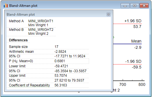
The coefficient of repeatability is not reported when you have selected the "Plot ratios" method.
Literature
- Abu-Arafeh A, Jordan H, Drummond G (2016) Reporting of method comparison studies: a review of advice, an assessment of current practice, and specific suggestions for future reports. British Journal of Anaesthesia 117:595-575.

- Barnhart HX, Barborial DP (2009) Applications of the repeatability of quantitative imaging biomarkers: a review of statistical analysis of repeat data sets. Translational Oncology 2:231-235.
- Bland JM, Altman DG (1986) Statistical method for assessing agreement between two methods of clinical measurement. The Lancet i:307-310.
- Bland JM, Altman DG (1995) Comparing methods of measurement: why plotting difference against standard method is misleading. The Lancet 346:1085-1087.
- Bland JM, Altman DG (1999) Measuring agreement in method comparison studies. Statistical Methods in Medical Research 8:135-160.
- CLSI (2013) Measurement procedure comparison and bias estimation using patient samples; Approved guideline - 3rd edition. CLSI document EP09-A3. Wayne, PA: Clinical and Laboratory Standards Institute.
- Gerke O (2020) Reporting Standards for a Bland–Altman Agreement Analysis: A Review of Methodological Reviews. Diagnostics 10, no. 5: 334.
- Hanneman SK (2008) Design, analysis, and interpretation of method-comparison studies. AACN Advanced Critical Care 19:223-234.
- Krouwer JS (2008) Why Bland-Altman plots should use X, not (Y+X)/2 when X is a reference method. Statistics in Medicine 27:778-780.
- Jensen AL, Kjelgaard-Hansen M (2010) Diagnostic test validation. In: Weiss D, Wardrop KJ, editors. Schalm's Veterinay Hematology, 6th ed. Ames: Wiley-Blackwell; p. 1027-1033.
- Stöckl D, Rodríguez Cabaleiro D, Van Uytfanghe K, Thienpont LM (2004) Interpreting method comparison studies by use of the Bland-Altman plot: reflecting the importance of sample size by incorporating confidence limits and predefined error limits in the graphic. Clinical Chemistry 50:2216-2218.