Weighted regression - worked example

The problem of heteroscedasticity

In regression analysis heteroscedasticity means a situation in which the variance of the dependent variable (Y) varies across the levels of the independent data (X). Heteroscedasticity can complicate analysis because regression analysis is based on an assumption of equal variance across the levels of the independent data.


Homoscedasticity	Heteroscedasticity

Weighted regression can be used to correct for heteroscedasticity. In a Weighted regression procedure more weight is given to the observations with smaller variance because these observations provide more reliable information about the regression function than those with large variances.

Neter et al. (1996). suggest the following process for estimating the regression coefficients in the presence of heteroscedasticity:

Fit the regression model by unweighted least squares and analyze the residuals.
Estimate the variance function or the standard deviation function by regressing either the squared residuals or the absolute residuals on the appropriate predictor(s).
Use the fitted values from the estimated variance or standard deviation function to obtain the weights w_i.
Estimate the regression coefficients using these weights.

How to do this automatically

MedCalc will perform these steps automatically when you select the dummy variable "*** AutoWeight 1/SD^2 ***" for "Weights" in the dialog boxes for regression.

How to perform each step in MedCalc

If you would like to have more control over the process, perhaps because you require some modifications of one or more steps, you can perform each of these steps using Weighted regression and other tools available in MedCalc.

This process is described below in detail.

The data for this example are available in the MedCalc sample files folder, file "Weighted regression (Neter).mc1". This file contains Age and Diastolic blood pressure (DBP) data collected on 54 subjects.

Weighted regression example data

Source

Step 1. Fit the regression model by unweighted least squares and analyze the residuals

We click Regression on the Statistics menu and complete the dialog box as follows.

Dialog box for regression (weighed regression example)

Variable Y, the dependent variable is DBP (Diastolic blood pressure) and Variable X, the independent variable is Age.

We do not select a variable for Weights because in this first step we perform ordinary unweighted least squares regression.

We obtain the following results:

Regression results (weighed regression example)

In the results window, we click the hyperlink "Save residuals" to save the residuals in a new column of the spreadsheet.

Residuals are the differences between the observed values of the dependent variable DBP and the values calculated using the regression equation.

Save residuals (weighed regression example)

In the subsequent dialog box, we click OK.

Save residuals (weighed regression example)

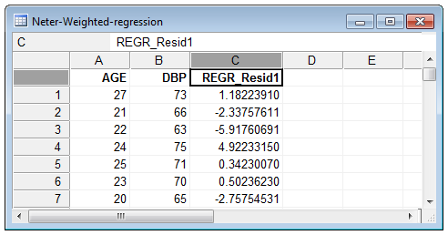
This will create a new column in the spreadsheet containing the residuals (variable "REGR_Resid1"):

Save residuals (weighed regression example)

Step 2. Estimate the variance function or the standard deviation function

In this step, we build a regression model of the standard deviation against Age. We do that by regressing the absolute values of the residuals against Age, since the absolute residuals are an estimator of the standard deviation of DBP at different values of Age.

We click Regression on the Statistics menu and complete the dialog box as follows:

Dialog box regression (weighted regression example)

For Variable Y, we first select the new variable "REGR_Resid1" and next edit the selection and change the variable into "abs(REGR_Resid1)".

We obtain the following results:

Regression results (weighted regression example)

Step 3. Use the fitted values from the estimated variance or standard deviation function to obtain the weights

In the last results window, we click the hyperlink "Save predicted values" to save the predicted values in a new column of the spreadsheet.

Save predicted values

In the subsequent dialog box, we click OK.

Save predicted values

This will create a new column in the spreadsheet containing the predicted (or estimated) values of the standard deviation (variable "REGR_Pred1"):

Predicted values saved in spreadsheet

Step 4. Estimate the regression coefficients using these weights

Finally, we can build our weighted regression model.

For weights we use the reciprocal of the squared predicted values for standard deviation (variance is the standard deviation squared): observations with large standard deviation are given less weight than observations with smaller standard deviation.

$$ weight = \frac{1}{SD^2} $$

We click Regression on the Statistics menu and complete the dialog box as follows.

Dialog box regression (weighted regression example)

For Weights, we first select the new variable "REGR_Pred1" and next edit the selection and change the variable into "1/REGR_Pred1^2" (we could also use "1/(REGR_Pred1*REGR_Pred1)" or "1/Power(REGR_Pred1,2)".

We obtain the following results:

Regression results (weighted regression example)

The final (weighted) regression equation is

DBP = 55.5658 + 0.5963 Age

which is not much different from the original (unweighted) regression equation

DBP = 56.1569 + 0.5800 Age

However, the standard errors of the regression coefficients are smaller, resulting in more narower confidence intervals.

Literature

Neter J, Kutner MH, Nachtsheim CJ, Wasserman W (1996) Applied linear statistical models. 4^th ed. Boston: McGraw-Hill.

Weighted regression - worked example

The problem of heteroscedasticity

How to do this automatically

How to perform each step in MedCalc

Step 1. Fit the regression model by unweighted least squares and analyze the residuals

Step 2. Estimate the variance function or the standard deviation function

Step 3. Use the fitted values from the estimated variance or standard deviation function to obtain the weights

Step 4. Estimate the regression coefficients using these weights

Literature

See also