Summary statistics
| Command: | Statistics |
Description
Allows to calculate summary statistics: mean, median, standard deviation, percentiles, etc.
Required input
In the Summary statistics dialog box you select the variable of interest. You can also enter a filter in the Select field, in order to include only a selected subgroup of cases, as described in the Introduction part of this manual.

You can click the ![]() button to obtain a list of variables. In this list you can select a variable by clicking the variable's name.
button to obtain a list of variables. In this list you can select a variable by clicking the variable's name.
Options
- Logarithmic transformation: if the data require a logarithmic transformation (e.g. when the data are positively skewed), select the Logarithmic transformation option.
- Test for Normal distribution: see Tests for Normal distribution.
- Click the More options button for additional options:

- Percentiles: allows to select the percentiles of interest.
- Other averages
- Trimmed mean: option to calculate a trimmed mean. You select the percentage of observations that will be trimmed away. For example, when you select 10% then the lowest 10% and highest 10% of observations will be dropped for the calculation of the trimmed mean. See Calculation of Trimmed Mean, SE and confidence interval for computational details.
- Geometric mean. The geometric mean is given by:
$$\left ( \prod_{i=1}^n{x_i} \right ) ^\tfrac1n = \sqrt[n]{x_1 x_2 \cdots x_n} = \exp\left[\frac1n\sum_{i=1}^n\ln x_i\right] $$This option is not available when Logarithmic transformation is selected (when Logarithmic transformation is selected, the reported mean already is the Geometric mean).
- Harmonic mean. The harmonic mean is given by:
$$\frac{n}{\frac1{x_1} + \frac1{x_2} + \cdots + \frac1{x_n}} = \frac{n}{\sum\limits_{i=1}^n \frac1{x_i}} $$This option is not available when Logarithmic transformation is selected.
- Subgroups: (optionally) select a categorical variable to break-up the data in several (max. 8) subgroups. Summary statistics will be given for all data and for all subgroups.
 $$\left ( \prod_{i=1}^n{x_i} \right ) ^\tfrac1n = \sqrt[n]{x_1 x_2 \cdots x_n} = \exp\left[\frac1n\sum_{i=1}^n\ln x_i\right] $$
 $$\frac{n}{\frac1{x_1} + \frac1{x_2} + \cdots + \frac1{x_n}} = \frac{n}{\sum\limits_{i=1}^n \frac1{x_i}} $$
Results
Variable | WEIGHT |
|---|
Sample size | 100 |
|---|---|
Lowest value | 59.0000 |
Highest value | 105.0000 |
Arithmetic mean | 77.0400 |
95% CI for the Arithmetic mean | 75.1377 to 78.9423 |
Median | 77.0000 |
95% CI for the median | 74.0000 to 79.0000 |
Variance | 91.9176 |
Standard deviation | 9.5874 |
Relative standard deviation | 0.1244 (12.44%) |
Standard error of the mean | 0.9587 |
Coefficient of Skewness | 0.3684 (P=0.1242) |
Coefficient of Kurtosis | -0.2175 (P=0.7336) |
Shapiro-Wilk test | W=0.9835 |
Percentiles |
| 95% Confidence interval |
|---|---|---|
2.5 | 60.0000 |
|
5 | 62.5000 | 59.0000 to 65.1396 |
10 | 65.5000 | 62.0539 to 67.7165 |
25 | 70.0000 | 68.0000 to 72.0000 |
75 | 83.5000 | 80.0000 to 86.0000 |
90 | 90.0000 | 86.0000 to 94.9461 |
95 | 94.5000 | 90.7207 to 99.8311 |
97.5 | 95.0000 |
|
| Box-and-Whisker plot |
Sample size: the number of cases n is the number of numeric entries for the variable that fulfill the filter.
The lowest value and highest value of all observations (range).
Arithmetic mean: the arithmetic mean $\bar{x}$ is the sum of all observations divided by the number of observations n:
 $$\begin{align}
\bar{x} & = \frac{x_1+x_2+\cdots +x_n}{n} \\
& = {1 \over n} \sum_{i=1}^{n}{x_i} \\
& = {1 \over n} \sum_{}^{}{x}
\end{align}$$
$$\begin{align}
\bar{x} & = \frac{x_1+x_2+\cdots +x_n}{n} \\
& = {1 \over n} \sum_{i=1}^{n}{x_i} \\
& = {1 \over n} \sum_{}^{}{x}
\end{align}$$
95% confidence interval (CI) for the mean: this is a range of values, calculated using the method described later (see Standard Error of the Mean), which contains the population mean with a 95% probability.
Median: when you have n observations, and these are sorted from smaller to larger, then the median is equal to the value with order number (n+1)/2. The median is equal to the 50th percentile. If the distribution of the data is Normal, then the median is equal to the arithmetic mean. The median is not sensitive to extreme values or outliers, and therefore it may be a better measure of central tendency than the arithmetic mean.
95% confidence interval (CI) for the median: this is a range of values that contains the population median with a 95% probability (Campbell & Gardner, 1988). This 95% confidence interval can only be calculated when the sample size is not too small.
Variance: the variance is the mean of the square of the differences of all values with the arithmetic mean. The variance (s2) is calculated using the formula:
Standard deviation: the standard deviation (s or SD) is the square root of the variance, and is a measure of the spread of the data:
 $$s = \sqrt{\frac{\sum_{}^{}{(x-\bar{x})^2}}{n-1}} $$
When the distribution of the observations is Normal, then it can be assumed that 95% of all observations are located in the interval mean - 1.96 SD to mean + 1.96 SD (for other values see table: Values of the Normal distribution).

This interval should not be confused with the smaller 95% confidence interval for the mean. The interval mean - 1.96 SD to mean + 1.96 SD represents a descriptive 95% confidence range for the individual observations, whereas the 95% CI for the mean represents a statistical uncertainty of the arithmetic mean.
Relative standard deviation (RSD): this is the standard deviation divided by the mean. If appropriate, this number can be expressed as a percentage by multiplying it by 100 to obtain the coefficient of variation.
Standard error of the mean (SEM): is calculated by dividing the standard deviation by the square root of the sample size.
The SEM is used to calculate confidence intervals for the mean. When the distribution of the observations is Normal, or approximately Normal, then there is 95% confidence that the population mean is located in the interval x̄ ± t SEM, with t taken from the t-distribution with n−1 degrees of freedom and a confidence of 95% (see table Values of the t-distribution). For large sample sizes, t is close to 1.96.
Skewness
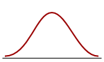
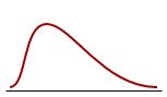
The coefficient of Skewness is a measure for the degree of symmetry in the variable distribution. If the corresponding P-value is low (P<0.05) then the variable symmetry is significantly different from that of a Normal distribution, which has a coefficient of Skewness equal to 0 (Sheskin, 2011).
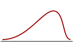 |  |  |
||
| Negatively skewed distribution or Skewed to the left Skewness <0 | Normal distribution Symmetrical Skewness = 0 | Positively skewed distribution or Skewed to the right Skewness > 0 |
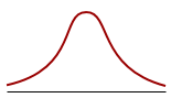
Kurtosis
The coefficient of Kurtosis is a measure for the degree of tailedness in the variable distribution (Westfall, 2014). If the corresponding P-value is low (P<0.05) then the variable tailedness is significantly different from that of a Normal distribution, which has a coefficient of Kurtosis equal to 0 (Sheskin, 2011).
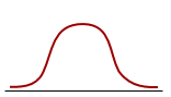 | |  |
||
| Platykurtic distribution Thinner tails Kurtosis <0 | Normal distribution Mesokurtic distribution Kurtosis = 0 | Leptokurtic distribution Fatter tails Kurtosis > 0 |
Test for Normal distribution: The result of this test is expressed as 'accept Normality' or 'reject Normality', with P value. If P is higher than 0.05, it may be assumed that the data have a Normal distribution and the conclusion 'accept Normality' is displayed.
If the P value is less than 0.05, then the hypothesis that the distribution of the observations in the sample is Normal, should be rejected, and the conclusion 'reject Normality' is displayed. In the latter case, the sample cannot accurately be described by arithmetic mean and standard deviation, and such samples should not be submitted to any parametric statistical test or procedure, such as e.g. a t-test. To test the possible difference between not Normally distributed samples, the Wilcoxon test can be used, and correlation can be estimated by means of rank correlation.
When the sample size is small, it may not be possible to perform the selected test and an appropriate message will appear. In this case you can visually evaluate the symmetry and peakedness of the distribution using the histogram or cumulative frequency distribution.
Percentiles (or "centiles"): when you have n observations, and these are sorted from smaller to larger, then the p-th percentile is equal to the observation with rank number (Lentner, 1982; Schoonjans et al., 2011):
When the rank number R(p) is a whole number, then the percentile coincides with the sample value; if R(p) is a fraction, then the percentile lies between the values with ranks adjacent to R(p) and in this case MedCalc uses interpolation to calculate the percentile.
The formula for R(p) is only valid when
E.g. the 5th and 95th percentiles can only be estimated when n ≥ 20, since
Therefore it makes no sense to quote the 5th and 95th percentiles when the sample size is less than 20. In this case it is advised to quote the 10th and 90th percentiles, at least if the sample size is not less than 10.
The percentiles can be interpreted as follows: p % of the observations lie below the p-th percentile, e.g. 10% of the observations lie below the 10th percentile.
The 25th percentile is called the 1st quartile, the 50th percentile is the 2nd quartile (and equals the Median), and the 75th percentile is the 3rd quartile.
The numerical difference between the 25th and 75 percentile is the interquartile range. Within the 2.5th and 97.5th percentiles lie 95% of the values and this range is called the 95% central range. The 90% central range is defined by the 5th and 95th percentiles, and the 10th and 90th percentiles define the 80% central range.
Logarithmic transformation
If the option Logarithmic transformation was selected, the program will display the back-transformed results. The back-transformed mean is named the Geometric mean. Variance, Standard deviation and Standard error of the mean cannot be back-transformed meaningfully and are not reported.
Presentation of results
The description of the data in a publication will include the sample size and arithmetic mean. The standard deviation can be given as an indicator of the variability of the data: the mean was 25.6 mm (SD 3.2 mm). The standard error of the mean can be given to show the precision of the mean: the mean was 25.6 mm (SE 1.6 mm).
When you want to make an inference about the population mean, you can give the mean and the 95% confidence interval of the mean: the mean was 25.6 (95% CI 22.4 to 28.8).
If the distribution of the variable is positively skewed, then a mathematical transformation of the data may be applied to obtain a Normal distribution, e.g. a logarithmic or square root transformation. After calculations you can convert the results back to the original scale. It is then useless to report the back-transformed standard deviation or standard error of the mean. Instead, you can antilog the confidence interval in case a logarithmic transformation was applied, or square the confidence interval if you have applied a square root transformation (Altman et al., 1983). The resulting confidence interval will then not be symmetrical, reflecting the shape of the distribution. If, for example, after logarithmic transformation of the data, the mean is 1.408 and the 95% confidence interval is 1.334 to 1.482, then you will antilog these statistics and report: the mean was 25.6 mm (95% CI 21.6 to 30.3).
If the distribution of the variable is not normal even after logarithmic or other transformation, then it is better to report the median and a percentiles range, e.g. the interquartile range, or the 90% or 95% central range: the median was 25.6 mm (95% central range 19.6 to 33.5 mm). The sample size will be taken into consideration when you decide whether to use the interquartile range or the 90% or 95% central range (see percentiles) (Altman, 1980).
The precision of the reported statistics should correspond to the precision of the original data. The mean and 95% CI can be given to one decimal place more than the raw data, the standard deviation and standard error can be given with one extra decimal (Altman et al., 1983).
Finally, the summary statistics in the text or table may be complemented by a graph (see distribution plots).
Literature
- Altman DG (1980) Statistics and ethics in medical research. VI - Presentation of results. British Medical Journal 281:1542-1544.

- Altman DG (1991) Practical statistics for medical research. London: Chapman and Hall.
- Altman DG, Gore SM, Gardner MJ, Pocock SJ (1983) Statistical guidelines for contributors to medical journals. British Medical Journal 286:1489-1493.
- Campbell MJ, Gardner MJ (1988) Calculating confidence intervals for some non-parametric analyses. British Medical Journal 296:1454-1456.
- Lentner C (ed) (1982) Geigy Scientific Tables, 8th edition, Volume 2. Basle: Ciba-Geigy Limited.
- Schoonjans F, De Bacquer D, Schmid P (2011) Estimation of population percentiles. Epidemiology 22: 750-751.
- Sheskin DJ (2011) Handbook of parametric and non-parametric statistical procedures. 5th ed. Boca Raton: Chapman & Hall /CRC.
- Westfall PH (2014) Kurtosis as Peakedness, 1905 - 2014. R.I.P. The American Statistician 68:191-195.
