Cox proportional-hazards regression
| Command: | Statistics |
Description
Cox regression (or Cox proportional hazards regression) is a statistical method to analyze the effect of several risk factors on survival, or in general on the time it takes for a specific event to happen.
The probability of the endpoint (death, or any other event of interest, e.g. recurrence of disease) is called the hazard. The hazard is modeled as:
where X1 ... Xk are a collection of predictor variables and H0(t) is the baseline hazard at time t, representing the hazard for a person with the value 0 for all the predictor variables.
By dividing both sides of the above equation by H0(t) and taking logarithms, we obtain:
We call H(t) / H0(t) the hazard ratio. The coefficients bi...bk are estimated by Cox regression, and can be interpreted in a similar manner to that of multiple logistic regression.
Suppose the covariate (risk factor) is dichotomous and is coded 1 if present and 0 if absent. Then the quantity exp(bi) can be interpreted as the instantaneous relative risk of an event, at any time, for an individual with the risk factor present compared with an individual with the risk factor absent, given both individuals are the same on all other covariates.
Suppose the covariate is continuous, then the quantity exp(bi) is the instantaneous relative risk of an event, at any time, for an individual with an increase of 1 in the value of the covariate compared with another individual, given both individuals are the same on all other covariates.
Required input

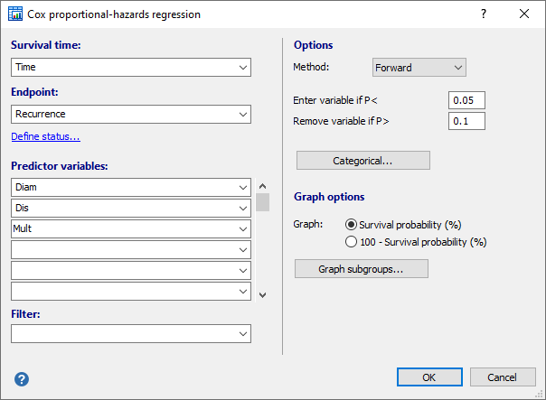
Survival time: The name of the variable containing the time to reach the event of interest, or the time of follow-up.
Endpoint: The name of a variable containing codes 1 for the cases that reached the endpoint, or code 0 for the cases that have not reached the endpoint, either because they withdrew from the study, or the end of the study was reached. If your data are coded differently, you can use the Define status tool to recode your data.
Predictor variables: Names of variables that you expect to predict survival time.
The Cox proportional regression model assumes that the effects of the predictor variables are constant over time. Furthermore there should be a linear relationship between the endpoint and predictor variables. Predictor variables that have a highly skewed distribution may require logarithmic transformation to reduce the effect of extreme values. Logarithmic transformation of a variable var can be obtained by entering LOG(var) as predictor variable.
Filter: A filter to include only a selected subgroup of cases in the graph.
Options
- Method: select the way independent variables are entered into the model.
- Enter: enter all variables in the model in one single step, without checking
- Forward: enter significant variables sequentially
- Backward: first enter all variables into the model and next remove the non-significant variables sequentially
- Stepwise: enter significant variables sequentially; after entering a variable in the model, check and possibly remove variables that became non-significant.
- Enter variable if P<
a variable is entered into the model if its associated significance level is less than this P-value. - Remove variable if P>
a variable is removed from the model if its associated significance level is greater than this P-value. - Categorical: click this button to identify categorical variables.
Graph options
- Graph:
- Survival probability (%): plot Survival probability (%) against time (descending curves)
- 100 - Survival probability (%): plot 100 - Survival probability (%) against time (ascending curves)
- Graph subgroups: here you can select one of the predictor variables. The graph will display different survival curves for all values in this covariate (which must be categorical, and may not contain more than 8 categories). If no covariate is selected here, then the graph will display the survival at mean of the covariates in the model.

Results
In the example (taken from Bland, 2000), "survival time" is the time to recurrence of gallstones following dissolution (variable Time). Recurrence is coded in the variable Recurrence (1= yes, 0 =No). Predictor variables are Dis (= number of months previous gallstones took to dissolve), Mult (1 in case of multiple previous gallstones, 0 in case of single previous gallstones), and Diam (maximum diameter of previous gallstones).
Survival time | Time |
|---|---|
Endpoint | Recurrence |
Method | Forward |
|---|---|
Enter variable if P< | 0.05 |
Remove variable if P> | 0.1 |
Cases summary
Number of events a | 39 | 27.08% |
|---|---|---|
Number censored b | 105 | 72.92% |
Total number of cases | 144 | 100.00% |
a Recurrence = 1
b Recurrence = 0
Overall Model Fit
Null model -2 Log Likelihood | 339.097 |
|---|---|
Full model -2 Log Likelihood | 326.933 |
Chi-squared | 12.164 |
DF | 2 |
Significance level | P = 0.0023 |
Coefficients and Standard Errors
Covariate | b | SE | Wald | P | Exp(b) | 95% CI of Exp(b) |
|---|---|---|---|---|---|---|
Dis | 0.04292 | 0.01657 | 6.7106 | 0.0096 | 1.0439 | 1.0105 to 1.0783 |
Mult | 0.9635 | 0.3528 | 7.4599 | 0.0063 | 2.6208 | 1.3127 to 5.2326 |
Variables not included in the model |
|---|
Diam |
Baseline cumulative hazard function
| Baseline | At mean of Covariates | |
|---|---|---|---|
Time | Cumulative Hazard | Cumulative Hazard | Survival |
6 | 0.011 | 0.030 | 0.971 |
7 | 0.016 | 0.043 | 0.958 |
8 | 0.025 | 0.065 | 0.937 |
9 | 0.028 | 0.073 | 0.930 |
10 | 0.031 | 0.081 | 0.922 |
11 | 0.040 | 0.105 | 0.900 |
12 | 0.057 | 0.150 | 0.861 |
13 | 0.061 | 0.160 | 0.852 |
16 | 0.069 | 0.182 | 0.833 |
17 | 0.073 | 0.194 | 0.824 |
18 | 0.082 | 0.218 | 0.804 |
19 | 0.087 | 0.231 | 0.794 |
24 | 0.094 | 0.247 | 0.781 |
25 | 0.100 | 0.264 | 0.768 |
26 | 0.106 | 0.281 | 0.755 |
28 | 0.113 | 0.299 | 0.741 |
29 | 0.127 | 0.336 | 0.714 |
30 | 0.142 | 0.376 | 0.687 |
32 | 0.151 | 0.400 | 0.671 |
38 | 0.168 | 0.444 | 0.641 |
43 | 0.201 | 0.529 | 0.589 |
60 | 0.302 | 0.796 | 0.451 |
Concordance
Harrell's C-index | 0.652 |
|---|---|
95% Confidence interval | 0.560 to 0.744 |
|
|
Save prognostic indices |
Cases summary
This table shows the number of cases that reached the endpoint (Number of events), the number of cases that did not reach the endpoint (Number censored), and the total number of cases.
Overall Model Fit
The Chi-squared statistic tests the relationship between time and all the covariates in the model.
Coefficients and Standard Errors
Using the Forward selection method, the two covariates Dis and Mult were entered in the model which significantly (0.0096 for Dis and 0.0063 for Mult) contribute to the prediction of time.
MedCalc lists the regression coefficient b, its standard error, Wald statistic (b/SE)2, P value, Exp(b) and the 95% confidence interval for Exp(b).
Exp(b) and Hazard ratio
- For a continuous covariate, Exp(b) is the increase of the hazard ratio for 1 unit change of the continuous variable.
When b is negative, then Exp(b) is less than 1 and Exp(b) is the decrease of the hazard ratio for 1 unit change of the continuous variable.
- For a dichotomous covariate, Exp(b) is the hazard ratio.
The coefficient for months for dissolution (continuous variable Dis) is 0.0429. Exp(b) = Exp(0.0429) is 1.0439 (with 95% Confidence Interval 1.0107 to 1.0781), meaning that for an increase of 1 month to dissolution of previous gallstones, the hazard ratio for recurrence increases by a factor 1.04. For 2 months the hazard ratio increases by a factor 1.042.
The coefficient for multiple gallstones (dichotomous variable Mult) is 0.9335. Exp(b) = Exp(0.9635) is 2.6208, meaning that a case with previous gallstones is 2.6208 (with 95% Confidence Interval 1.3173 to 5.2141) more likely to have a recurrence than a case with a single stone.
Variables not included in the model
The variable Diam was found not to significantly contribute to the prediction of time, and was not included in the model.
Baseline cumulative hazard function
Finally, the program lists the baseline cumulative hazard H0(t), with the cumulative hazard and survival at mean of all covariates in the model.
The baseline cumulative hazard can be used to calculate the survival probability S(t) for any case at time t:
where PI is a prognostic index:
Concordance
Harrell's C-index (Harrell et al., 1996), also known as the concordance index, is a goodness of fit measure for models which produce risk scores. See Park et al. (2021) for a detailed description.
Values of C near 1 indicate that the cox regression model is good at predicting which of 2 patients will take longer to present the event of interest. Values of C near 0.5 indicate that the model is no better than a coin flip in determining which patient will present the event of interest first. Values near 0 means that the model performs worse than a coin flip.
The confidence interval of Harrell's C-index is calculated using the modified τ method according to Pencina (2004).
Graph
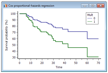
The graph displays the survival curves for all categories of the categorical variable Mult (1 in case of multiple previous gallstones, 0 in case of single previous gallstones), and for mean values for all other covariates in the model.

If no covariate was selected for Graph - Subgroups, or if the selected variable was not included in the model, then the graph displays a single survival curve at mean of all covariates in the model.
Sample size considerations
Based on the work of Peduzzi et al. (1995) the following guideline for a minimum number of cases to include in a study can be suggested.
Let p be the smallest of the proportions of positive cases (cases that reached the endpoint) and negative cases (cases that did not reach the endpoint) in the population and k the number of predictor variables, then the minimum number of cases to include is:
N = 10 k / p
For example: you have 3 predictor variables to include in the model and the proportion of positive cases in the population is 0.20 (20%). The minimum number of cases required is
N = 10 x 3 / 0.20 = 150
If the resulting number is less than 100 you should increase it to 100 as suggested by Long (1997).
Literature
- Christensen E (1987) Multivariate survival analysis using Cox's regression model. Hepatology 7:1346-1358.
- Harrell FE Jr, Lee KL, Mark DB (1996) Multivariable prognostic models: issues in developing models, evaluating assumptions and adequacy, and measuring and reducing errors. Statistics in Medicine 15:361-387.
- Long JS (1997) Regression Models for categorical and limited dependent variables. Thousand Oaks, CA: Sage Publications.
- Park SY, Park JE, Kim H, Park SH (2021) Review of statistical methods for evaluating the performance of survival or other time-to-event prediction models (from conventional to deep learning approaches). Korean Journal of Radiology.
- Peduzzi P, Concato J, Feinstein AR, Holford TR (1995) Importance of events per independent variable in proportional hazards regression analysis. II. Accuracy and precision of regression estimates. Journal of Clinical Epidemiology 48:1503-1510.
- Pencina MJ, D'Agostino RB (2004) Overall C as a measure of discrimination in survival analysis: model specific population value and confidence interval estimation. Statistics in Medicine 23:2109-2123.
- Rosner B (2006) Fundamentals of Biostatistics. 6th ed. Pacific Grove: Duxbury.
 $$\ln \left( { \operatorname{H}(t) \over \operatorname{H}_0(t)}\right) = b_1 X_1 + b_2 X_2 + b_3 X_3 + \cdots + b_k X_k$$
